Optimization methods in Scipy

Mathematical optimization is the selection of the best input in a function to compute the required value. In the case we are going to see, we'll try to find the best input arguments to obtain the minimum value of a real function, called in this case, cost function. This is called minimization.

In the next examples, the functions scipy.optimize.minimize_scalar and scipy.optimize.minimize will be used. The examples can be done using other Scipy functions like scipy.optimize.brent or scipy.optimize.fmin_{method_name}, however, Scipy recommends to use the minimize and minimize_scalar interface instead of these specific interfaces.

Finding a global minimum can be a hard task. Scipy provides different stochastic methods to do that, but it won't be covered in this article.

Let's start:

import numpy as np
from scipy import optimize, special
import matplotlib.pyplot as plt

1D optimization

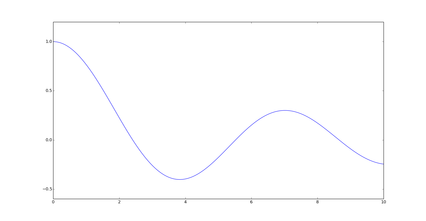
For the next examples we are going to use the Bessel function of the first kind of order 0, here represented in the interval (0,10].

x = np.linspace(0, 10, 500)
y = special.j0(x)
plt.plot(x, y)
plt.show()

Golden section method minimizes a unimodal function by narrowing the range in the extreme values:

optimize.minimize_scalar(special.j0, method='golden')

  fun: -0.40275939570255315
    x: 3.8317059773846487
 nfev: 43

Brent's method is a more complex algorithm combination of other root-finding algorithms:

optimize.minimize_scalar(special.j0, method='brent')

  fun: -0.40275939570255309
 nfev: 10
  nit: 9
    x: 3.8317059554863437

plt.plot(x, y)
plt.axvline(3.8317059554863437, linestyle='--', color='k')
plt.show()

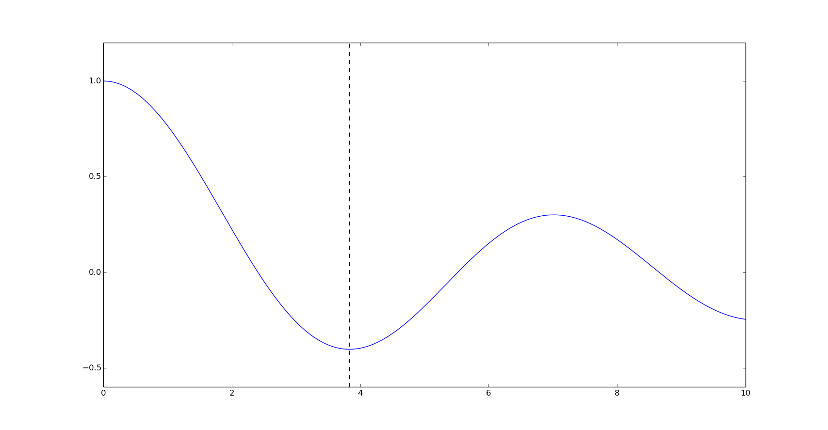
As we can see in this example, Brent method minimizes the function in less objective function evaluations (key nfev) than the Golden section method.

Multivariate optimization

The Rosenbrock function is widely used for tests performance in optimization algorithms. The Rosenbrock function has a parabolic-shaped valley with the global minimum in it.

The function definition is:

It has a global minimum at $(x,y)=(a,a^2)$, where $f(x,y)=0$.

Scipy provides a multidimensional Rosenbrock function, a variant defined as:

x, y = np.mgrid[-2:2:100j, -2:2:100j]
plt.pcolor(x, y, optimize.rosen([x, y]))
plt.plot(1, 1, 'xw')
plt.colorbar()
plt.axis([-2, 2, -2, 2])
plt.title('Rosenbrock function')
plt.xlabel('x')
plt.ylabel('y')
plt.show()

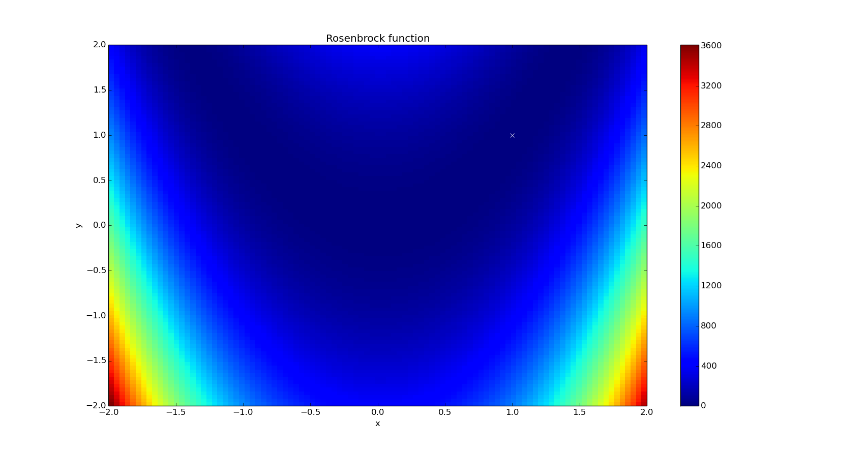
For the next examples, we are going to use it as a 2D function, with a global minimum found at (1,1).

Initial guess:

x0 = (0., 0.)

Gradient-less optimization

Nelder-Mead and Powell methods are used to minimize functions without the knowledge of the derivative of the function, or gradient.

Nelder-Mead method, also known as downhill simplex is an heuristics method to converge in a non-stationary point:

optimize.minimize(optimize.rosen, x0, method='Nelder-Mead')

  status: 0
    nfev: 146
 success: True
     fun: 3.6861769151759075e-10
       x: array([ 1.00000439,  1.00001064])
 message: 'Optimization terminated successfully.'
     nit: 79

Powel's conjugate direction method is an algorithm where the minimization is achieved by the displacement of vectors by a search for a lower point:

optimize.minimize(optimize.rosen, x0, method='Powell')

  status: 0
 success: True
   direc: array([[  1.54785007e-02,   3.24539372e-02],
       [  1.33646191e-06,   2.53924992e-06]])
    nfev: 462
     fun: 1.9721522630525295e-31
       x: array([ 1.,  1.])
 message: 'Optimization terminated successfully.'
     nit: 16

As we can see in this case, Powell's method finds the minimum in less steps (iterations, key nit), but with more function evaluations than Nelder-Mead method. Modifying the initial direction of the vectors we may get a better result with less function evaluations. Let's try setting and initial direction of (1,0) from our initial guess, (0,0):

optimize.minimize(
    optimize.rosen, x0, method='Powell', options={'direc': (1, 0)})

  status: 0
 success: True
   direc: array([ 1.,  0.])
    nfev: 52
     fun: 0.0
       x: array([ 1.,  1.])
 message: 'Optimization terminated successfully.'
     nit: 2

We'll find the minimum in considerably less function evaluations of the different points.

Sometimes we can use gradient methods, like BFGS, without knowing the gradient:

optimize.minimize(optimize.rosen, x0, method='BFGS')

   status: 2
  success: False
     njev: 32
     nfev: 140
 hess_inv: array([[ 0.48552643,  0.96994585],
       [ 0.96994585,  1.94259477]])
      fun: 1.9281078336062298e-11
        x: array([ 0.99999561,  0.99999125])
  message: 'Desired error not necessarily achieved due to precision loss.'
      jac: array([ -1.07088609e-05,   5.44565446e-06])

In this case, we haven't achieved the optimization. We will see more about gradient-based minimization in the next section.

Gradient-based optimization

These methods will need the derivatives of the cost function, in the case of the Rosenbrock function, the derivative is provided by Scipy, anyway, here's the simple calculation in Maxima:

rosen: (1-x)^2 + 100*(y-x^2)^2;

rosen_d: [diff(rosen, x), diff(rosen, y)];

Conjugate gradient method is similar to a simpler gradient descent but it uses a conjugate vector and in each iteration the vector moves in a direction conjugate to the all previous steps:

optimize.minimize(optimize.rosen, x0, method='CG', jac=optimize.rosen_der)

  status: 0
 success: True
    njev: 33
    nfev: 33
     fun: 6.166632297117924e-11
       x: array([ 0.99999215,  0.99998428])
 message: 'Optimization terminated successfully.'
     jac: array([ -7.17661535e-06,  -4.26162510e-06])

BFGS calculates an approximation of the hessian of the objective function in each iteration, for that reason it is a Quasi-Newton method (more on Newton method later):

optimize.minimize(optimize.rosen, x0, method='BFGS', jac=optimize.rosen_der)

   status: 0
  success: True
     njev: 26
     nfev: 26
 hess_inv: array([[ 0.48549325,  0.96988373],
       [ 0.96988373,  1.94247917]])
      fun: 1.1678517168020135e-16
        x: array([ 1.00000001,  1.00000002])
  message: 'Optimization terminated successfully.'
      jac: array([ -2.42849398e-07,   1.30055966e-07])

BFGS achieves the optimization on less evaluations of the cost and jacobian function than the Conjugate gradient method, however the calculation of the hessian can be more expensive than the product of matrices and vectors used in the Conjugate gradient.

L-BFGS is a low-memory aproximation of BFGS. Concretely, the Scipy implementation is L-BFGS-B, which can handle box constraints using the bounds argument:

optimize.minimize(optimize.rosen,
                  x0,
                  method='L-BFGS-B',
                  jac=optimize.rosen_der)

  status: 0
 success: True
    nfev: 25
     fun: 1.0433892998247468e-13
       x: array([ 0.99999971,  0.9999994 ])
 message: 'CONVERGENCE: NORM_OF_PROJECTED_GRADIENT_<=_PGTOL'
     jac: array([  4.74035377e-06,  -2.66444085e-06])
     nit: 21

Hessian-based optimization

Newton's method uses the first and the second derivative (jacobian and hessian) of the objective function in each iteration.

This is the hessian matrix of the Rosenbrock function, calculated with Maxima:

rosen_d2: [[diff(rosen_d[1], x), diff(rosen_d[1], y)],
           [diff(rosen_d[2], x), diff(rosen_d[2], y)]];

Minimization Rosenbrock function using Newton's method with jacobian and hessian matrix:

optimize.minimize(optimize.rosen,
                  x0,
                  method='Newton-CG',
                  jac=optimize.rosen_der,
                  hess=optimize.rosen_hess)

  status: 0
 success: True
    njev: 85
    nfev: 53
     fun: 1.4946283615394615e-09
       x: array([ 0.99996137,  0.99992259])
 message: 'Optimization terminated successfully.'
    nhev: 33
     jac: array([ 0.01269975, -0.00637599])

Here we don't have a lower evaluations than the previous methods but we can use Newton's method for twice-differentiable quadratic functions to get faster results.