Least squares fitting with Numpy and Scipy

Nov 11, 2015 numerical-analysis numpy optimization python scipy

Both Numpy and Scipy provide black box methods to fit one-dimensional data using linear least squares, in the first case, and non-linear least squares, in the latter. Let's dive into them:

import numpy as np
from scipy import optimize
import matplotlib.pyplot as plt

Linear least squares fitting

Our linear least squares fitting problem can be defined as a system of m linear equations and n coefficents with m > n. In a vector notation, this will be:

X = [\begin{matrix} x_{11} & x_{12} & \dots & x_{1 n} \\ x_{21} & x_{22} & \dots & x_{2 n} \\ ⋮ & ⋮ & ⋱ & ⋮ \\ x_{m 1} & x_{m 2} & \dots & x_{m n} \end{matrix}], β = [\begin{matrix} β_{1} \\ β_{2} \\ ⋮ \\ β_{n} \end{matrix}], y = [\begin{matrix} y_{1} \\ y_{2} \\ ⋮ \\ y_{m} \end{matrix}]

The $X$ matrix corresponds to a Vandermonde matrix of our x variable, but in our case, instead of the first column, we will set our last one to ones in the variable a. Doing this and for consistency with the next examples, the result will be the array [m, c] instead of [c, m] for the linear equation

y = m x + c .

To get our best estimated coefficients we will need to solve the minimization problem

\hat{β} = \underset{β}{a r g m i n} ∥ y - X β ∥^{2}

by solving the equation

\hat{β} = (X^{T} X)^{- 1} X^{T} y

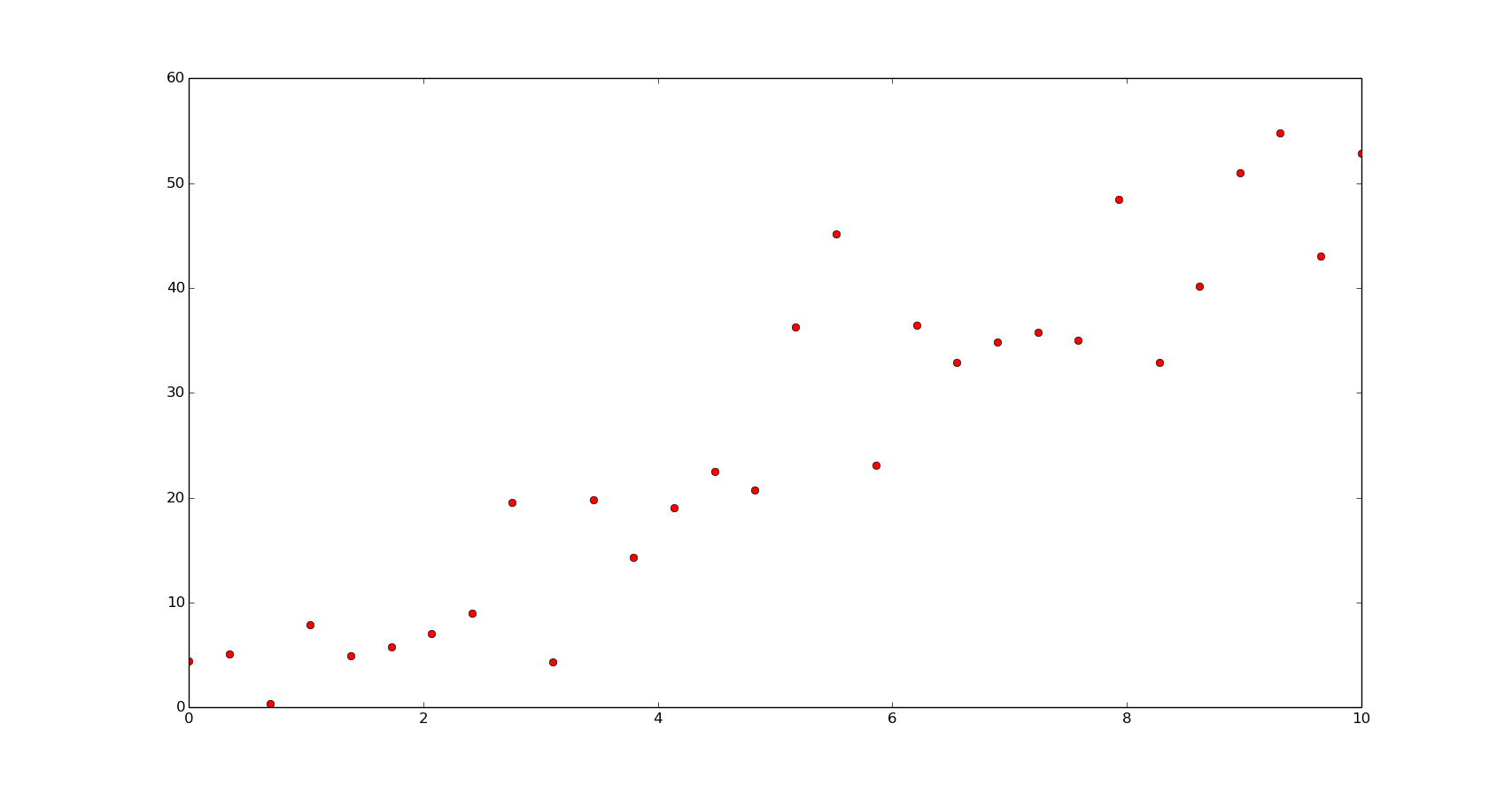
We can do this directly with Numpy. Let's create an example of noisy data first:

f = np.poly1d([5, 1])

x = np.linspace(0, 10, 30)
y = f(x) + 6*np.random.normal(size=len(x))
xn = np.linspace(0, 10, 200)

plt.plot(x, y, 'or')
plt.show()

Linear function data

To solve the equation with Numpy:

a = np.vstack([x, np.ones(len(x))]).T
np.dot(np.linalg.inv(np.dot(a.T, a)), np.dot(a.T, y))

array([ 5.59418256, -1.37189559])

We can use the lstsqs function from the linalg module to do the same:

np.linalg.lstsq(a, y)[0]

array([ 5.59418256, -1.37189559])

And, easier, with the polynomial module:

np.polyfit(x, y, 1)

array([ 5.59418256, -1.37189559])

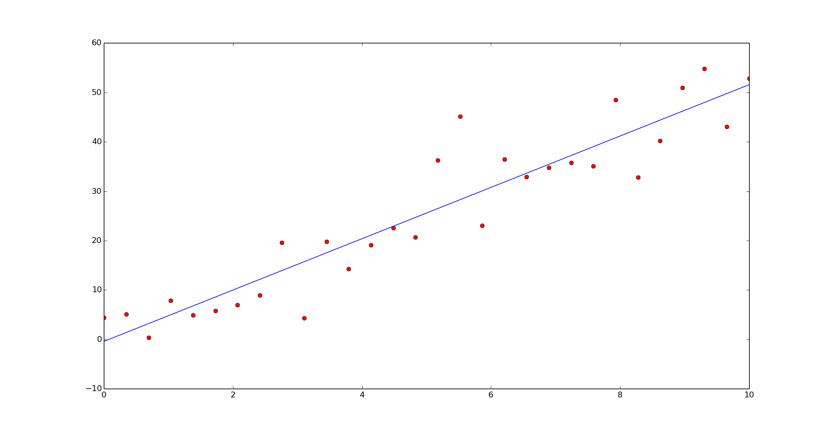
As we can see, all of them calculate a good aproximation to the coefficients of the original function.

m, c = np.polyfit(x, y, 1)
yn = np.polyval([m, c], xn)

plt.plot(x, y, 'or')
plt.plot(xn, yn)
plt.show()

Linear function data fit

In terms of speed, the first method is the fastest and the last one, a bit slower than the second method:

def leastsq1(x):
    a = np.vstack([x, np.ones(len(x))]).T
    return np.dot(np.linalg.inv(np.dot(a.T, a)), np.dot(a.T, y))

def leastsq2(x):
    a = np.vstack([x, np.ones(len(x))]).T
    return np.linalg.lstsq(np.vstack([x, np.ones(len(x))]).T, y)[0]

def leastsq3(x):
    return np.polyfit(x, y, 1)

%timeit leastsq1(x)

The slowest run took 8.36 times longer than the fastest. This could mean that an intermediate result is being cached
100000 loops, best of 3: 16 µs per loop

%timeit leastsq2(x)

The slowest run took 5.15 times longer than the fastest. This could mean that an intermediate result is being cached
10000 loops, best of 3: 58.8 µs per loop

%timeit leastsq3(x)

The slowest run took 4.43 times longer than the fastest. This could mean that an intermediate result is being cached
10000 loops, best of 3: 73.1 µs per loop

Polynomial fitting

In the case of polynomial functions the fitting can be done in the same way as the linear functions. Using polyfit, like in the previous example, the array x will be converted in a Vandermonde matrix of the size (n, m), being n the number of coefficients (the degree of the polymomial plus one) and m the lenght of the data array.

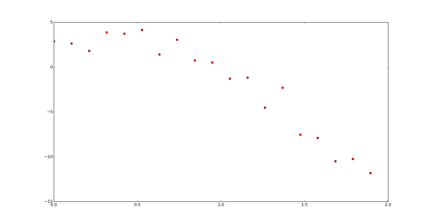
Just to introduce the example and for using it in the next section, let's fit a polynomial function:

f = np.poly1d([-5, 1, 3])
x = np.linspace(0, 2, 20)
y = f(x) + 1.5*np.random.normal(size=len(x))
xn = np.linspace(0, 2, 200)

plt.plot(x, y, 'or')
plt.show()

Polynomial function data

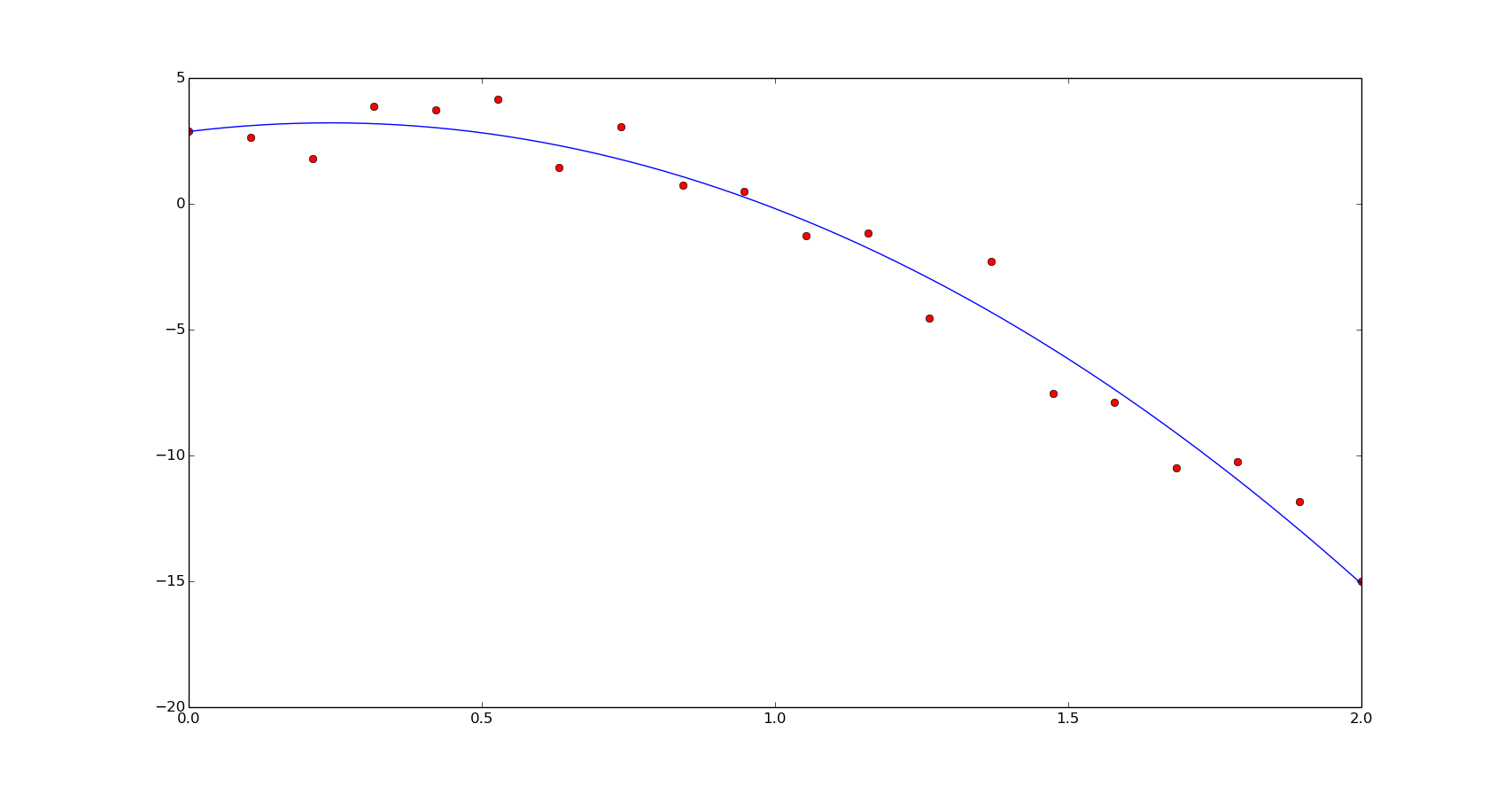
popt = np.polyfit(x, y, 2)
print popt

[-4.23466637 -1.0709698   4.51393962]

yn = np.polyval(popt, xn)

plt.plot(x, y, 'or')
plt.plot(xn, yn)
plt.show()

Polynomial function data linear fit

The speed results:

%timeit np.polyfit(x, y, 2)

The slowest run took 5.03 times longer than the fastest. This could mean that an intermediate result is being cached
10000 loops, best of 3: 79.4 µs per loop

Non-linear fitting

In this section we are going back to the previous post and make use of the optimize module of Scipy to fit data with non-linear equations.

Scipy's least square function uses Levenberg-Marquardt algorithm to solve a non-linear leasts square problems. Levenberg-Marquardt algorithm is an iterative method to find local minimums. We'll need to provide a initial guess ( $β$ ) and, in each step, the guess will be estimated as $β + δ$ determined by

f (x_{i}, β + δ) \approx f (x_{i}, β) + J_{i} δ,

being $J_{i}$ the gradient of the cost function with respect $β$ .

This gradient will be zero at the minimum of the sum squares and then, the coefficients ( $β$ ) will be the best estimated. In vector notation:

\underset{β + δ}{a r g m i n} ∥ y - f (β) - J δ ∥^{2} = 0.

This will be solved as:

(J^{T} J + λ diag (J^{T} J)) δ = J^{T} [y - f (β)],

being $λ$ the dumping factor (factor argument in the Scipy implementation).

Here is the implementation of the previous example. A function definition is used instead of the previous polynomial definition for a better performance and the residual function corresponds to the function to minimize the error, $y - f (β)$ in the previous equation:

def f(x, a, b, c):
    return a*x**2 + b*x + c

def residual(p, x, y):
    return y - f(x, *p)

p0 = [1., 1., 1.]
popt, pcov = optimize.leastsq(residual, p0, args=(x, y))

print popt

[-5.98229569  3.14299536  2.16551107]

yn = f(xn, *popt)

plt.plot(x, y, 'or')
plt.plot(xn, yn)
plt.show()

Polynomial function data non-linear fit

In terms of speed, we'll have similar results to the linear least squares in this case:

%timeit optimize.leastsq(residual, p0, args=(x, y))

10000 loops, best of 3: 79.3 µs per loop

In the following examples, non-polynomial functions will be used and the solution of the problems must be done using non-linear solvers. Also, we will compare the non-linear least square fitting with the optimizations seen in the previous post.

Exponential functions

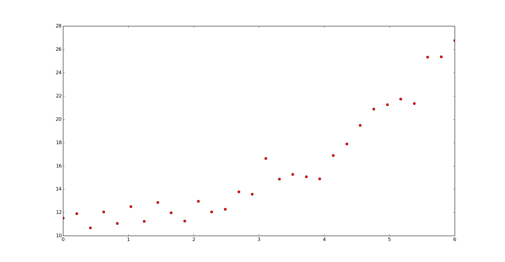
Here is the data we are going to work with:

def f(x, b, c):
    return b**x+c

p = [1.6, 10]
x = np.linspace(0, 6, 20)
y = f(x, *p) + np.random.normal(size=len(x))
xn = np.linspace(0, 6, 200)

plt.plot(x, y, 'or')
plt.show()

Exponential function data

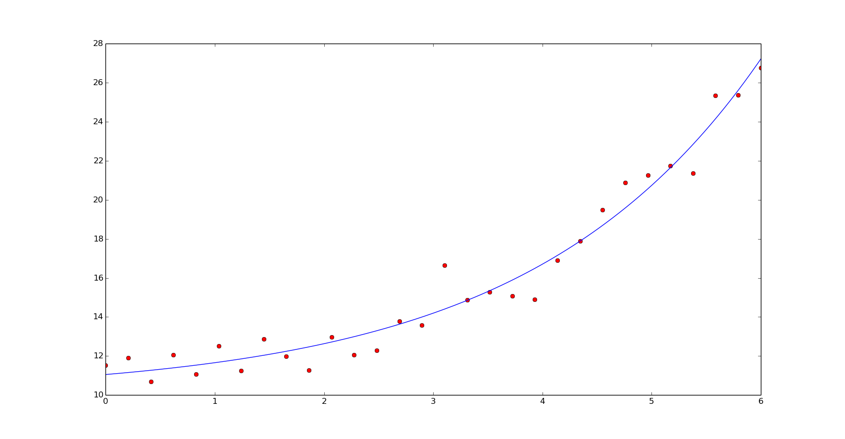
The non-linear least squares fit:

def residual(p, x, y):
    return y - f(x, *p)

p0 = [1., 8.]
popt, pcov = optimize.leastsq(residual, p0, args=(x, y))

print popt

yn = f(xn, *popt)

plt.plot(x, y, 'or')
plt.plot(xn, yn)
plt.show()

[  1.60598173  10.05263527]

Exponential function data fit

We should use non-linear least squares if the dimensionality of the output vector is larger than the number of parameters to optimize. Here, we can see the number of function evaluations of our last estimation of the coeffients:

popt, pcov, info, mesg, ler = optimize.leastsq(residual, p0, args=(x, y), full_output=True)
print info['nfev']

Using as a example, a L-BFGS minimization we will achieve the minimization in more cost function evaluations:

def min_residual(p, x, y):
    return sum(residual(p, x, y)**2)

res = optimize.minimize(min_residual, p0, method='L-BFGS-B', args=(x, y))
print res.x
print res.nfev

[  1.60598173  10.05263545]
60

An easier interface for non-linear least squares fitting is using Scipy's curve_fit. curve_fit uses leastsq with the default residual function (the same we defined previously) and an initial guess of [1.]*n, being n the number of coefficients required (number of objective function arguments minus one):

popt, pcov = optimize.curve_fit(f, x, y)
print popt

[  1.60598173  10.05263527]

In the speed comparison we can see a better performance for the leastqs function:

%timeit optimize.leastsq(residual, p0, args=(x, y))

1000 loops, best of 3: 166 µs per loop

%timeit optimize.curve_fit(f, x, y, p0=p0)

1000 loops, best of 3: 277 µs per loop

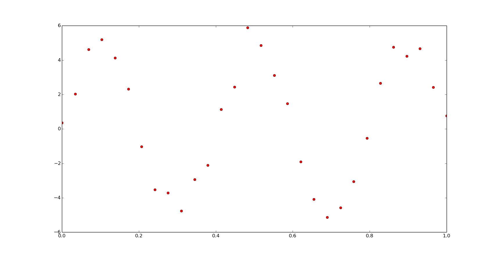
Trigonometric functions

Let's define some noised data from a trigonometric function:

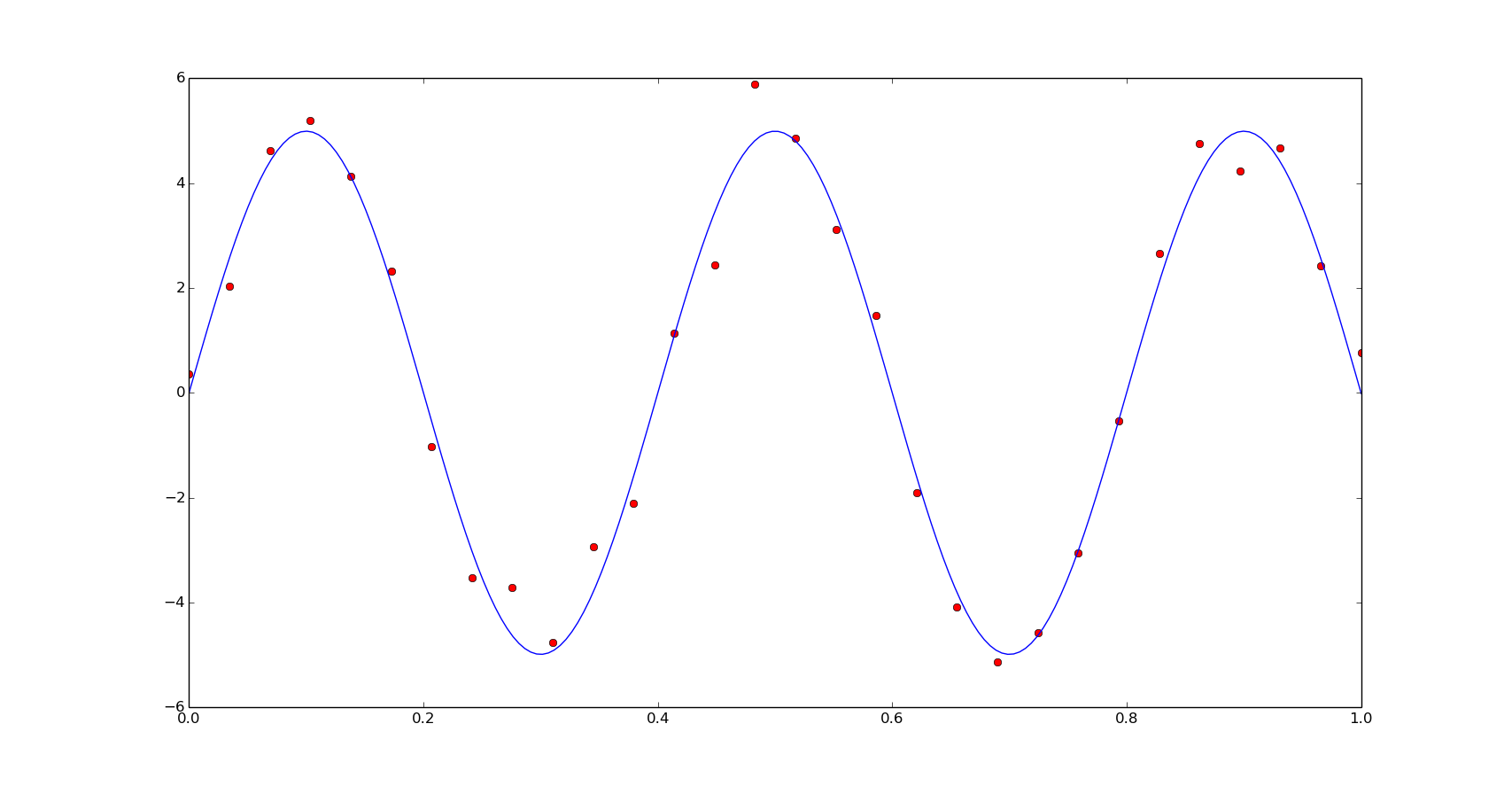
def f(x, a, b):
    return a*np.sin(b*np.pi*x)

p = [5, 5]
x = np.linspace(0, 1, 30)
y = f(x, *p) + .5*np.random.normal(size=len(x))
xn = np.linspace(0, 1, 200)

plt.plot(x, y, 'or')
plt.show()

Trigonometric function data

Fitting the data with non-linear least squares:

popt, pcov = optimize.curve_fit(f, x, y)

print popt

plt.plot(x, y, 'or')
plt.plot(xn, f(xn, *popt))
plt.show()

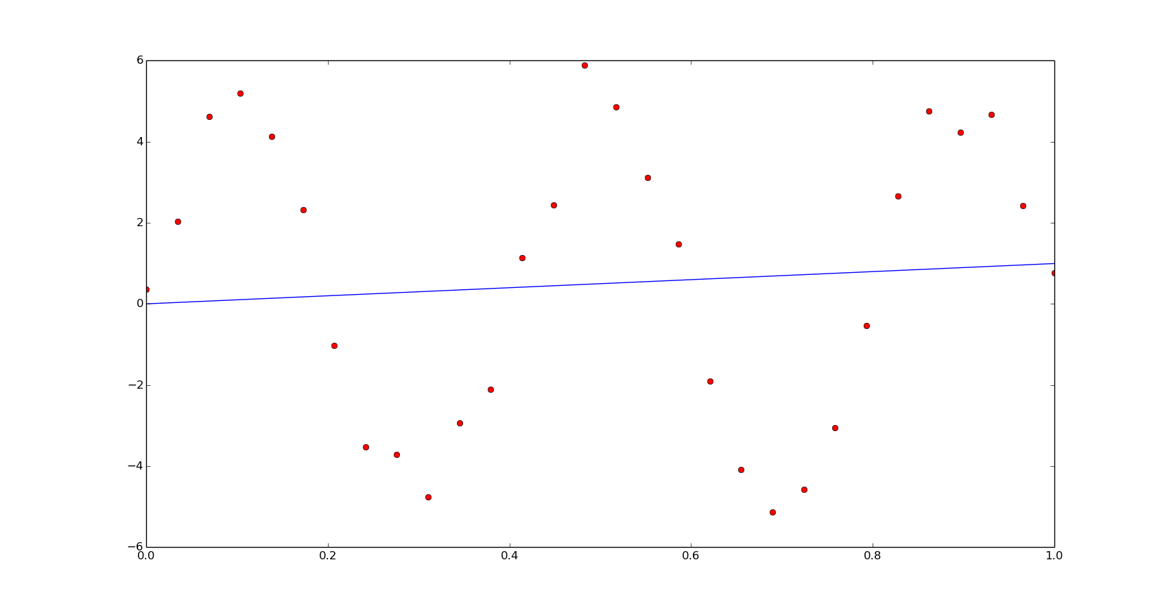
Trigonometric function data bad fit

We obtained a really bad fitting, in this case we will need a better initial guess. Observing the data we have it is possible to set a better initial estimation:

p0 = [3, 4]
popt, pcov = optimize.curve_fit(f, x, y, p0=p0)
print popt

plt.plot(x, y, 'or')
plt.plot(xn, f(xn, *popt))
plt.show()

Trigonometric function data fit

And the speed comparison for this function we observe similar results than the previous example:

%timeit optimize.leastsq(residual, p0, args=(x, y))

10000 loops, best of 3: 163 µs per loop

%timeit optimize.curve_fit(f, x, y, p0=p0)

1000 loops, best of 3: 281 µs per loop