Interpolation methods in Scipy

Among other numerical analysis modules, scipy covers some interpolation algorithms as well as a different approaches to use them to calculate an interpolation, evaluate a polynomial with the representation of the interpolation, calculate derivatives, integrals or roots with functional and class-based interfaces.

Let's see some interpolation examples for one and two-dimensional data.

First of all, the required modules:

import numpy as np
from scipy import interpolate
import matplotlib.pyplot as plt

Univariate interpolation

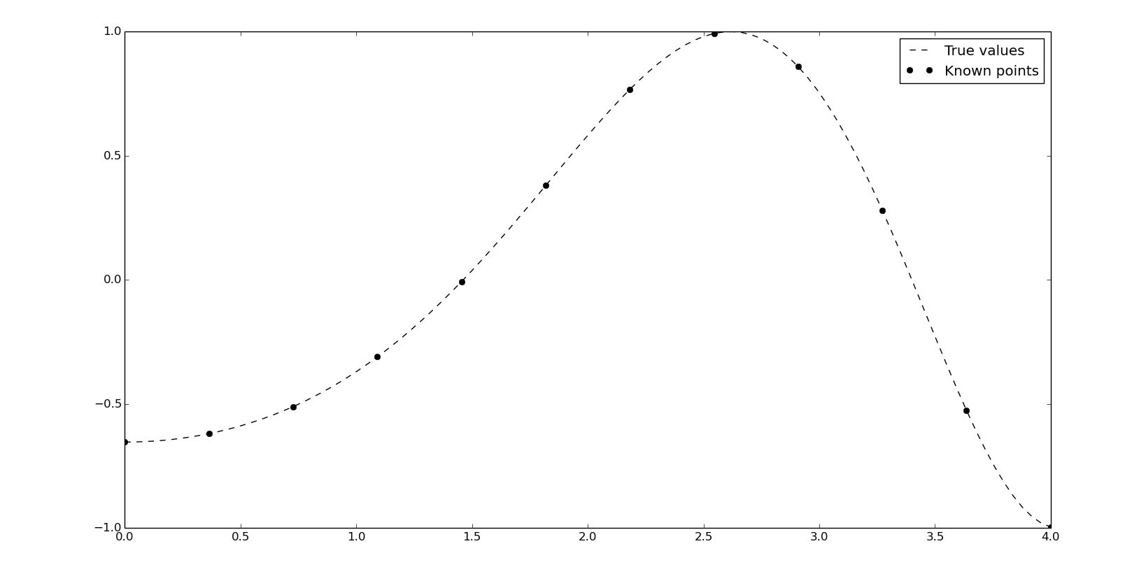
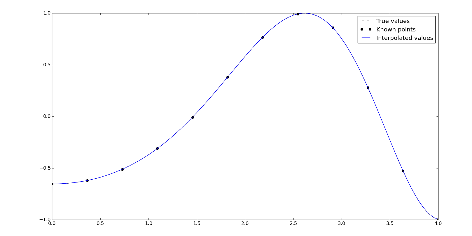
In the next examples, x and y represents the known points. We will need to obtain the interpolated values yn for xn. As a representation, y0 will be the true values, generated from the original function to show the interpolator behavior.

If nothing about the plots is said, they will be generated as:

plt.plot(xn, y0, '--k', label='True values')
plt.plot(x, y, 'ok', label='Known points')
plt.plot(xn, yn, label='Interpolated values')
plt.legend()
plt.show()

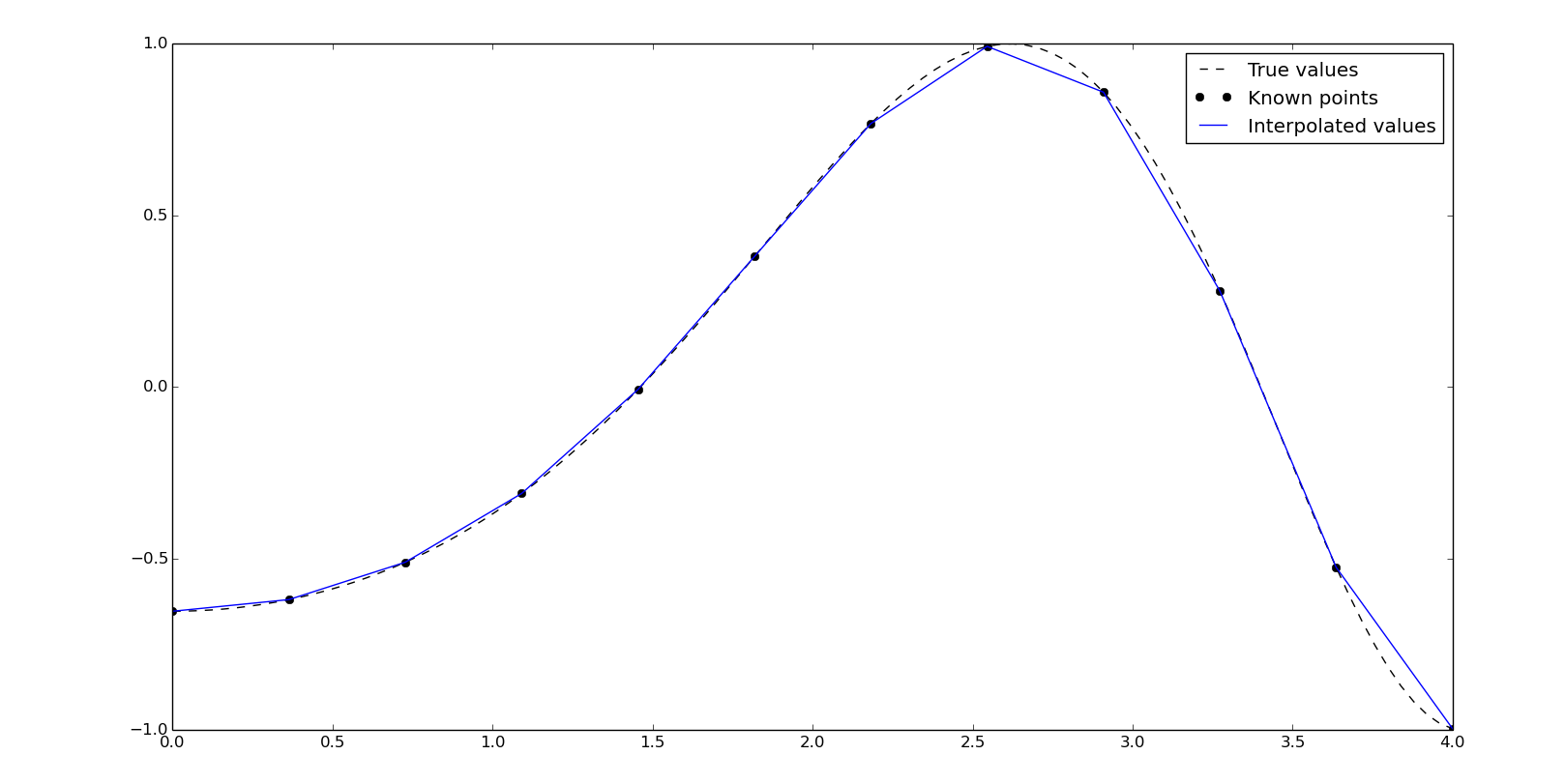
Linear interpolation

The linear interpolation is easy to compute but not precise, due to the discontinuites at the points.

We'll do some examples with this values:

x = np.linspace(0, 4, 12)
y = np.cos(x**2/3+4)

xn = np.linspace(0, 4, 100)
y0 = np.cos(xn**2/3+4)

We can compute a linear interpolation with numpy:

yn = np.interp(xn, x, y)

It's time to introduce the scipy's one-dimension interpolate class. The (interp1d)[http://docs.scipy.org/doc/scipy/reference/generated/scipy.interpolate.interp1d.html#scipy.interpolate.interp1d] object will be created from the known points and we can obtain yn evaluating itself with the corresponding xn. interp1d offers different interpolation methods by the kind argument and the default is linear:

f = interpolate.interp1d(x, y, kind='linear')
yn = f(xn)

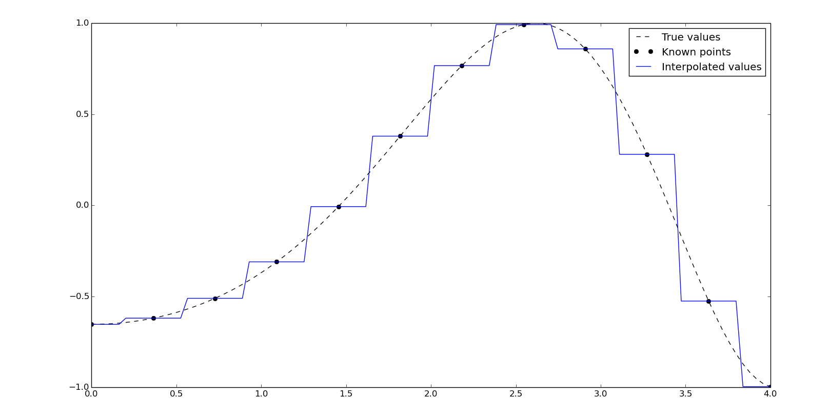
Nearest-neighbor interpolation

The univariate nearest-neighbor interpolation takes the same value of the closest known point:

f = interpolate.interp1d(x, y, kind='nearest')
yn = f(xn)

Polynominal interpolation

Polynominal interpolation algorithms are computationally expensive and can present oscillator artifacts in the extremes due to the Runge's phenomenon. Due to this, it is much better idea the use of Chebyshev polynomials or interpolate using splines (more later).

Lagrange or Newton are examples of polynomial interpolation. Just to mention and to introduce different interpolation problems approaches in scipy, let's see the Lagrange interpolation:

f = interpolate.lagrange(x, y)
yn = f(xn)

The barycentric interpolation uses Lagrange polynomials. We can calculate the interpolated values directly with the interpolation functions:

yn = interpolate.barycentric_interpolate(x, y, xn)

Alternativelly, we can use the class-based interpolators to generate a polynomial from the known points and then, call this polynomial with our xn data:

f = interpolate.BarycentricInterpolator(x, y)
yn = f(xn)

The use of the class-based approach is recommended if we need to evaluate the xn data more than once, since we already have our polynomial calculated.

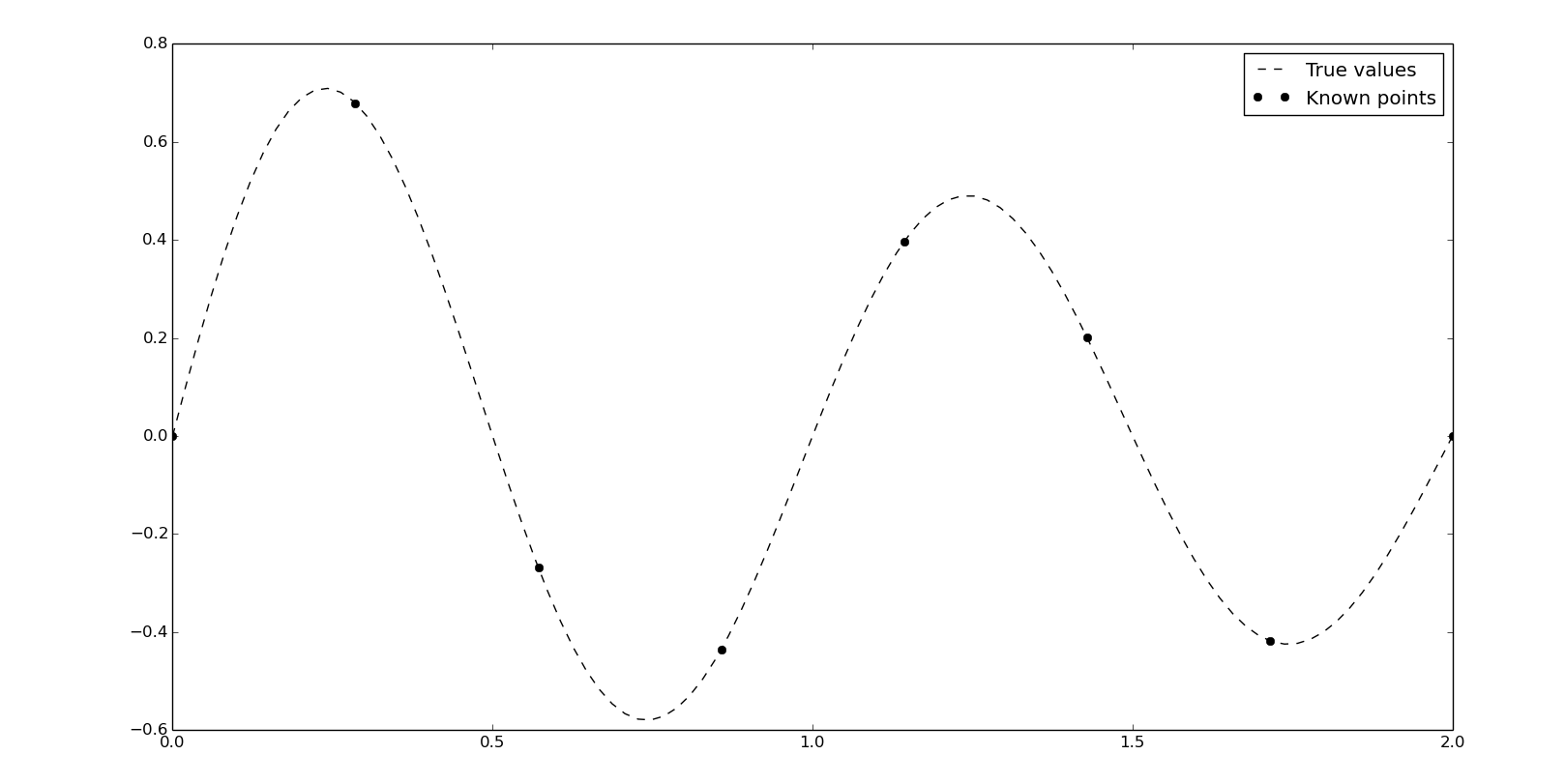
Splines

A spline is composed of polynomial functions connected by knots and, unlike the polynomial interpolation, does not present Runge's phenomenon, making the spline interpolation a stable and extended method of interpolation.

Let's change our data:

x = np.linspace(0, 2, 8)
y = 10*np.sinc(x*2+4)

xn = np.linspace(0, 2, 100)
y0 = 10*np.sinc(xn*2+4)

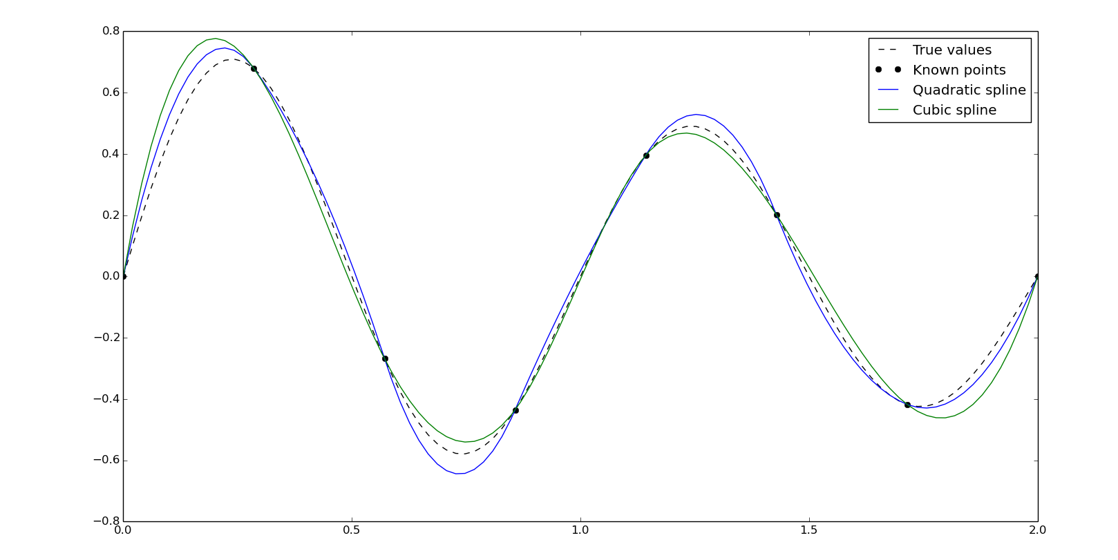
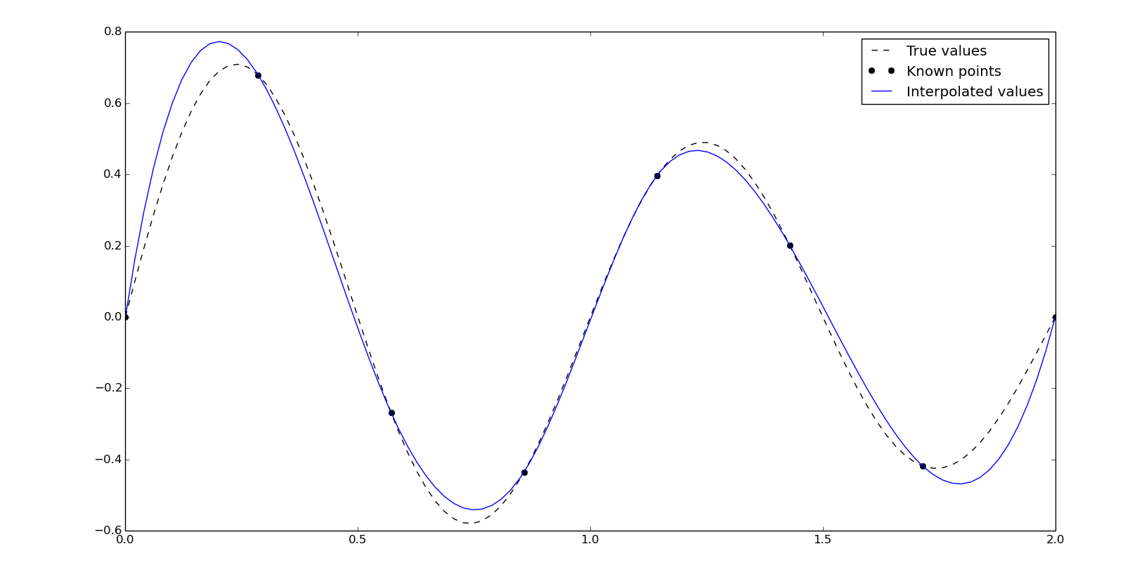
The easiest way to use splines in scipy is, again, with interp1d. Setting kind as quadratic or cubic we'll calculate the second and third order spline:

fq = interpolate.interp1d(x, y, kind='quadratic')
ynq = fq(xn)
fc = interpolate.interp1d(x, y, kind='cubic')
ync = fc(xn)

plt.plot(xn, y0, '--k', label='True values')
plt.plot(x, y, 'ok', label='Known points')
plt.plot(xn, ynq, label='Quadratic spline')
plt.plot(xn, ync, label='Cubic spline')
plt.legend()
plt.show()

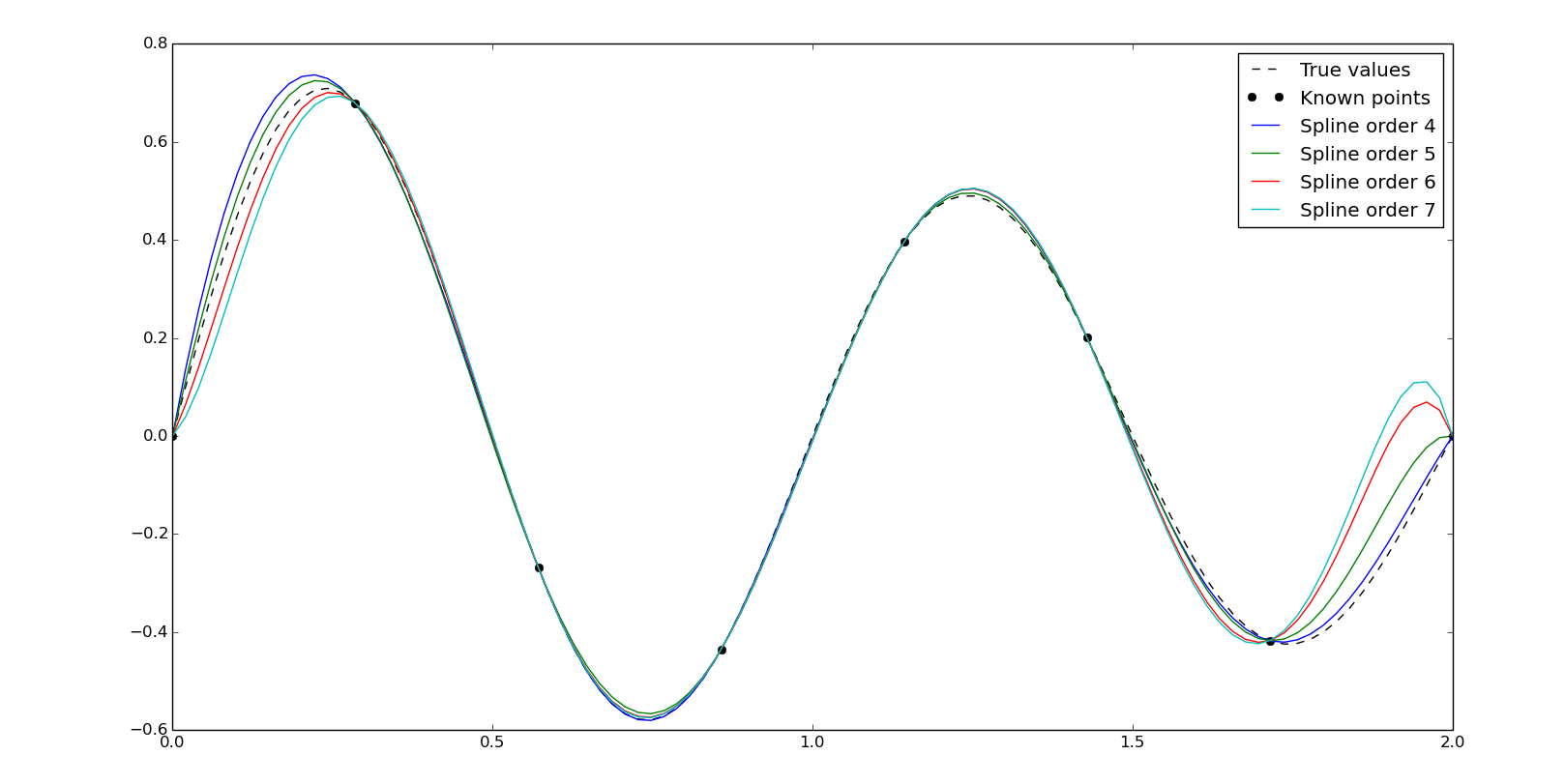
Specifying an integer as a kind we'll set the order of the polynomials, taking into account that the order has to be lower than the number of known points:

f4 = interpolate.interp1d(x, y, kind=4)
yn4 = f4(xn)
f5 = interpolate.interp1d(x, y, kind=5)
yn5 = f5(xn)
f6 = interpolate.interp1d(x, y, kind=6)
yn6 = f6(xn)
f7 = interpolate.interp1d(x, y, kind=7)
yn7 = f7(xn)

plt.plot(xn, y0, '--k', label='True values')
plt.plot(x, y, 'ok', label='Known points')
plt.plot(xn, yn4, label='Spline order 4')
plt.plot(xn, yn5, label='Spline order 5')
plt.plot(xn, yn6, label='Spline order 6')
plt.plot(xn, yn7, label='Spline order 7')
plt.legend()
plt.show()

Hermite polynomial is related to Newton polynomial, it is a divided derivatives calculation. Matches de value of the n points and the and its first m derivatives, so the resulting polynomial will have a degree of, at most, n(m+1)-1.

The cubic Hermite interpolation consists in a spline of third-degree Hermite polymonials and the Hermite curves can be specified as Bézier curves, widely used in vectorial graphics design.

In scipy, the cubic Hermite interpolation has the two different approaches presented in the previous section, the functional interpolation:

yn = interpolate.pchip_interpolate(x, y, xn)

and the class-based interpolator:

f = interpolate.PchipInterpolator(x, y)
yn = f(xn)

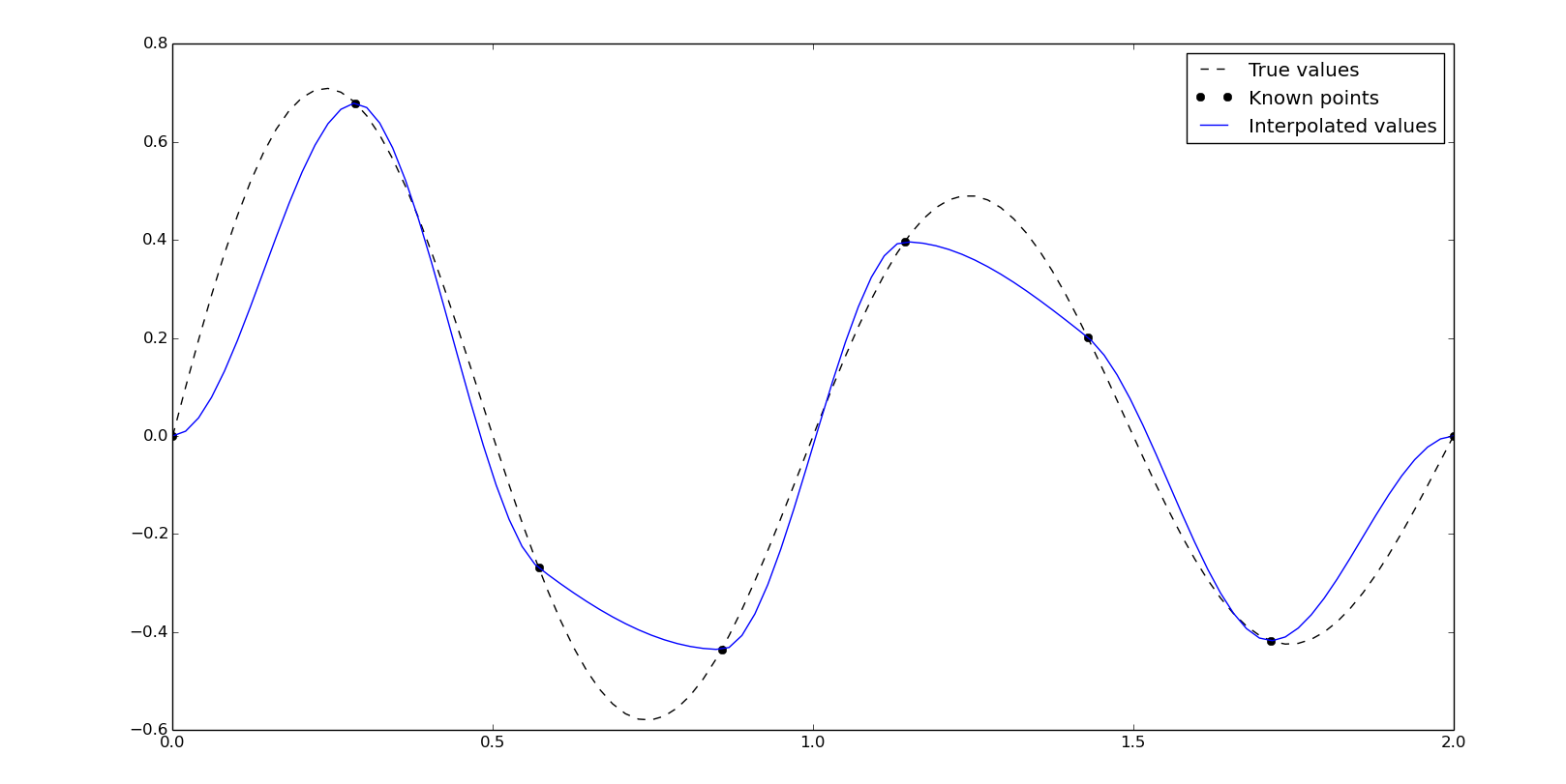
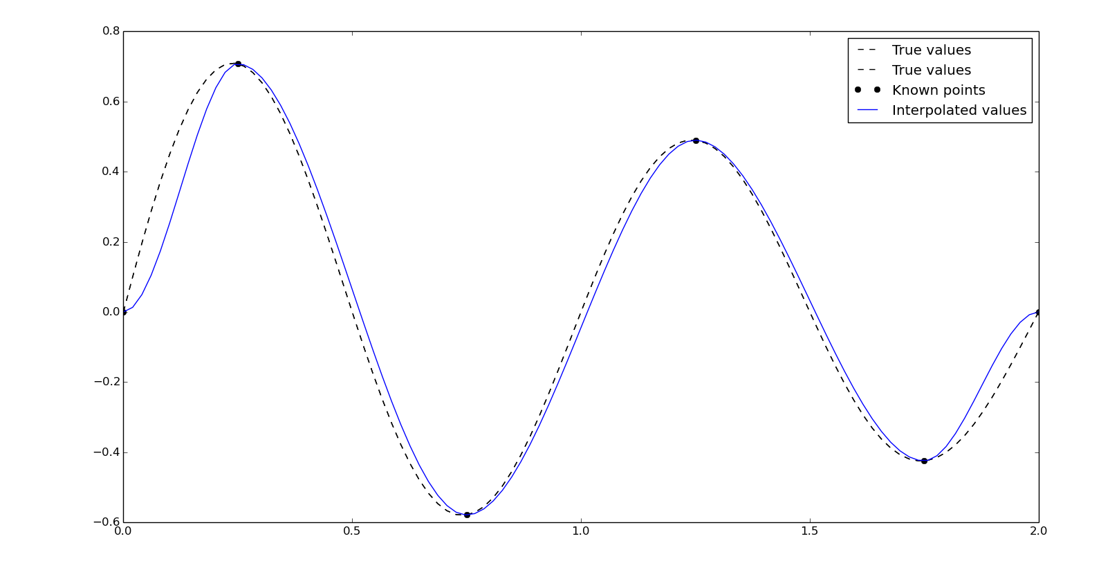
As we can see, the interpolated values are quite different than the true values. Like in vectorial graphic design, the points needed for the Bézier curve has to be more significative, so in this case, we need to locate points in local maximimums or minimums. For the sinc function Asinc(Bx+C) we will find the peaks close to 1/2B, due to the C parameter, and then, close to every 1/2B, in this case {0.25, 0.75, 1.25, 1.75}. So, using the next points we will get a better result using the cubic Hermite interpolation:

x2 = np.array([0, .25, .75, 1.25, 1.75, 2])
y2 = 10*np.sinc(x2*2+4)
yn = interpolate.pchip_interpolate(x2, y2, xn)

Splines can also be calculated using the class-based interpolator, In this case with the FITPACK interface:

spline = interpolate.InterpolatedUnivariateSpline(x, y, k=3)
yn = spline(xn)

And through the FITPACK functional interface:

# Get spline representation (knots, coefficients and degree).
tck = interpolate.splrep(x, y, k=3)
# Evaluate spline and its derivatives.
yn = interpolate.splev(xn, tck)

In both cases we will have many evaluation methods, for example, getting the roots of the function:

print spline.roots()

[  4.60185838e-17   4.91329683e-01   1.00253142e+00   1.51200452e+00]

With FITPACK functional interface:

print interpolate.sproot(tck)

[  4.60185838e-17   4.91329683e-01   1.00253142e+00   1.51200452e+00]

By the definition of the sinc function Asinc(Bx+C), roots will be found at every 1/B and at 0, due to the C parameter, which for the interval (0,2] will be {0, 0.5, 1, 1.5}.

Multivariate interpolation

Multivariate interpolation refers to a spatial interpolation, to functions with more than one variable. It is mainly used in image processing (bilinear interpolation) and geology elevation models (Kriging interpolation, not covered here).

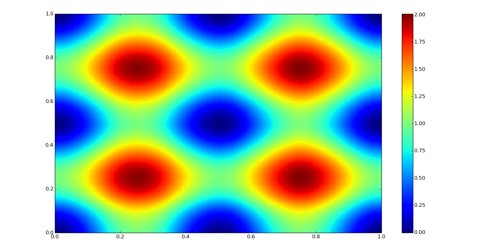
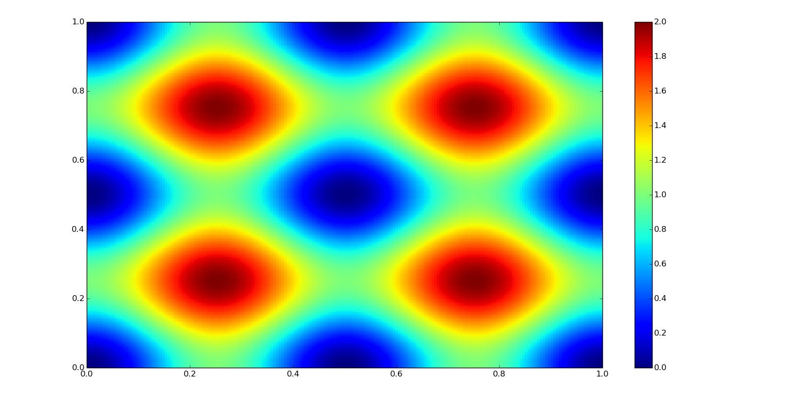
First, let's go to define some data: xn and yn are the coordinates where we are going to interpolate our data, this coordinates are defined as well as a meshgrid (numpy.mgrid); z0 corresponds to the true values for the coordinates; and f0, the function to define it (both, unknown in the practice).

def f0(x, y):
    return np.sin(2*np.pi*x)**2 + np.sin(2*np.pi*y)**2

grid_xn, grid_yn = np.mgrid[0:1:200j, 0:1:200j]
xn = grid_xn[:,0]
yn = grid_yn[0,:]
z0 = f0(grid_xn, grid_yn)

plt.pcolor(grid_xn, grid_yn, z0)
plt.colorbar()
plt.show()

In the next examples, if nothing is said, the interpolation results will be displayed as a pseudocolor map as:

plt.pcolor(grid_xn, grid_yn, zn)
plt.colorbar()
plt.show()

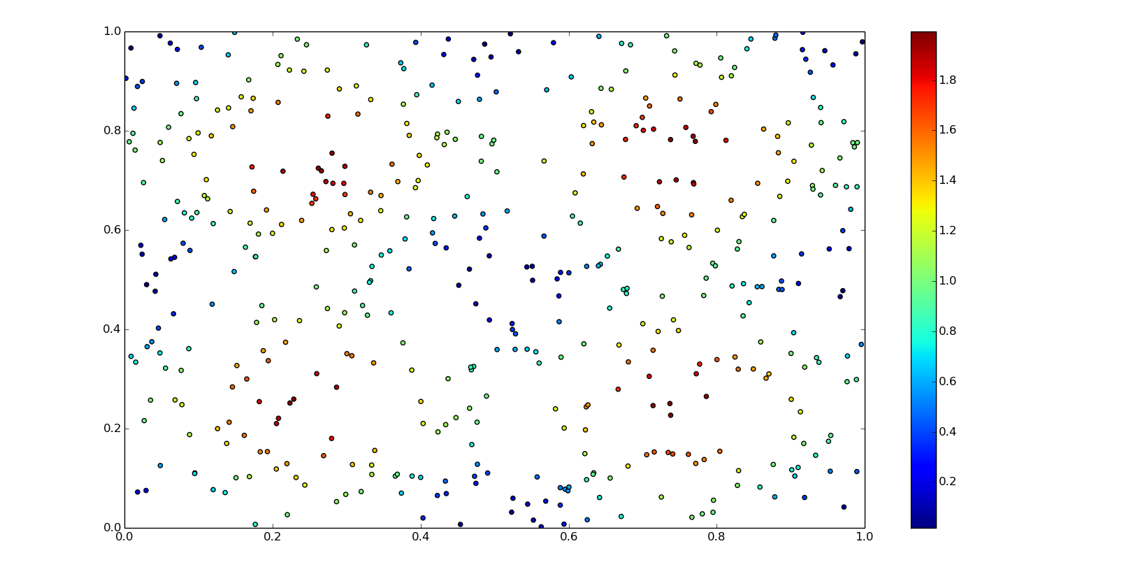
For the next example we neeed to create some unstructured data, an array of points and the corresponding values:

points = np.random.rand(500, 2)
values = f0(points[:, 0], points[:, 1])

plt.scatter(points[:, 0], points[:, 1], c=values)
plt.colorbar()
plt.axis([0,1,0,1])
plt.show()

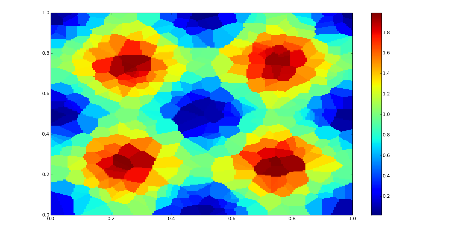
Two-dimensional nearest-neighbor interpolation

Multivariate nearest-neighbor is not computationally expensive, so it is used in real-time three dimensional rendering. The concept is equivalent to Voronoi diagram.

Class-based interpolator:

f = interpolate.NearestNDInterpolator(points, values)
zn = f(grid_xn, grid_yn)

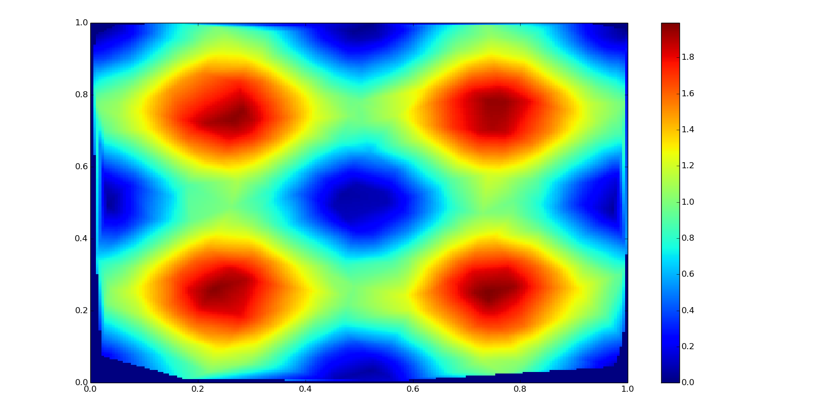
Bilinear interpolation

A bilinear interpolation is based in two linear interpolations in a 2D grid. It is used in image resampling.

Class-based interpolator:

f = interpolate.LinearNDInterpolator(points, values, fill_value=0)
zn = f(grid_xn, grid_yn)

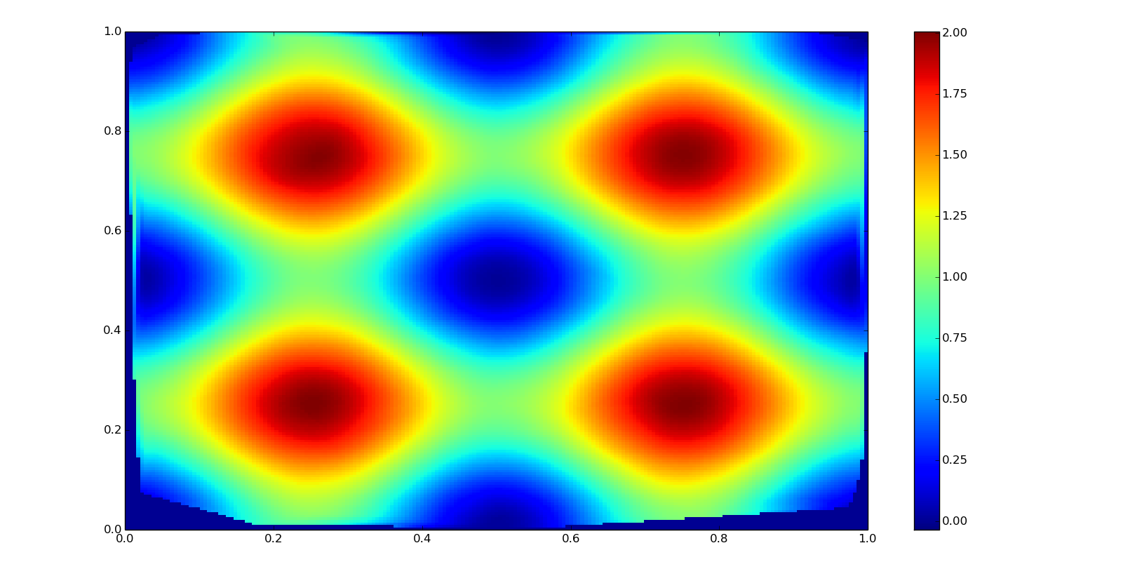
Bicubic spline interpolation

It is based in two splines of order three in a two-dimensional grid. Used in image processing and GIS altitude data. It is smoother than bilinear and nearest-neighbor interpolation but more computationally expensive.

In this case we are going to use scpiy.interpolate.griddata function, which creates directly a grid with the interpolated values in a similar way as interp1d. This function supports also linear and nearest-neighbor interpolations in two dimensions with the method argument.

zn = interpolate.griddata(
    points, values, (grid_xn, grid_yn), fill_value=0, method='cubic')

More about multivariate splines

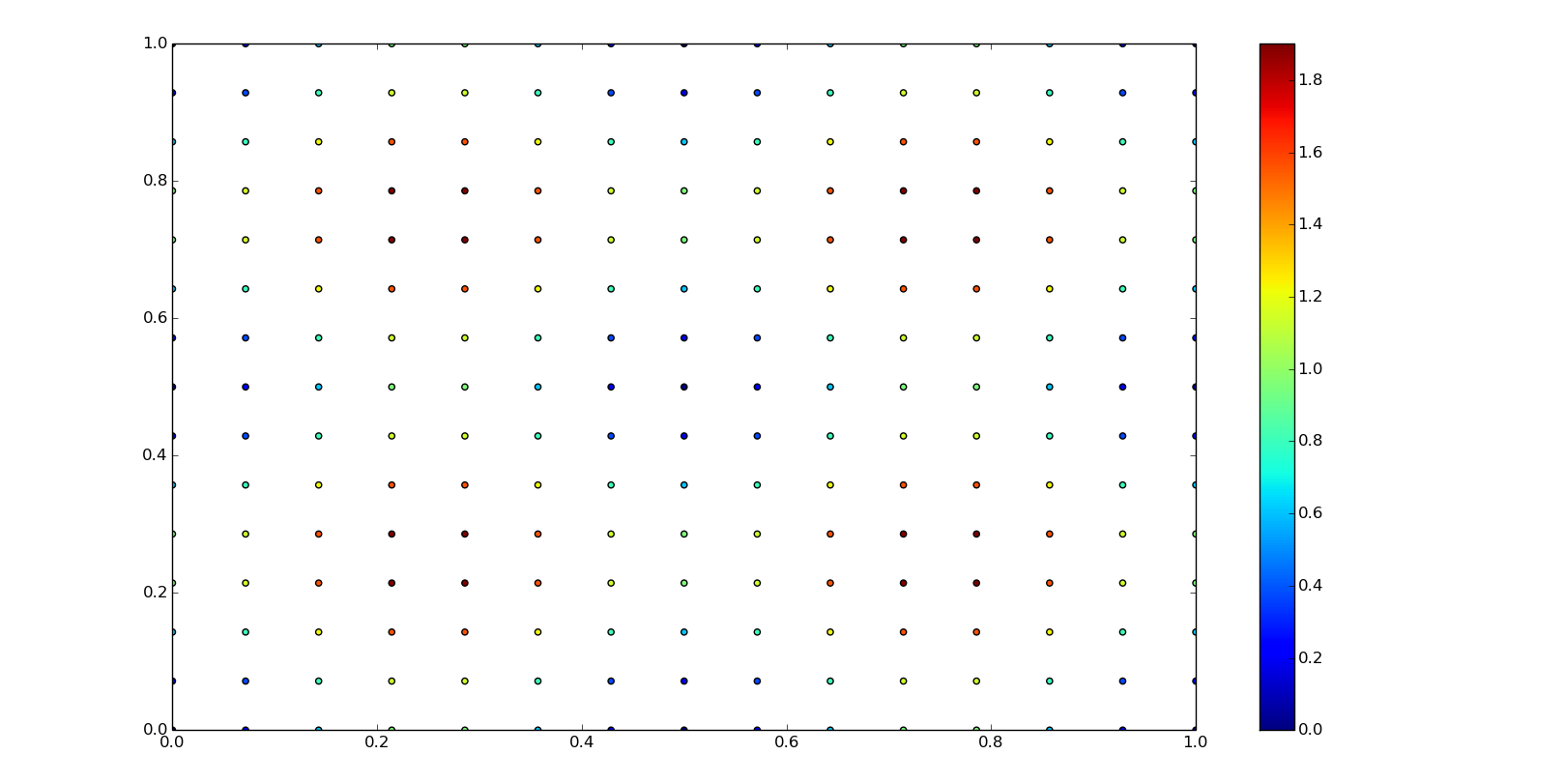
For the next examples we are going to need some structured data, values in a grid corresponding to ranked x an y coordinates:

grid_x, grid_y = np.mgrid[0:1:15j, 0:1:15j]
x = grid_x[:, 0]
y = grid_y[0, :]
z = f0(grid_x, grid_y)

plt.scatter(grid_x, grid_y, c=z)
plt.axis([0,1,0,1])
plt.colorbar()
plt.show()

Similar to the functional FITPACK interface for one-dimesional splines, here's the representation and evaluation of a bicubic spline using points and values as a grid data:

tck = interpolate.bisplrep(grid_x, grid_y, z, s=0, kx=3, ky=3)
zn = interpolate.bisplev(xn, yn, tck)

And the same with the class-based FITPACK interface. In this case we will need to calculate the spline with points not as a grid but as a ranked arrays:

spline = interpolate.RectBivariateSpline(x, y, z, s=0, kx=3, ky=3)
zn = spline(xn, yn)