Image affine mapping in Numpy

Previously, we implemented linear transformations to a matrix in Numpy. In this case we will apply an affine transformation to an image, mapping three points to the new origin, top right and bottom left corner.

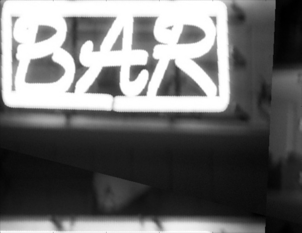
The image (source) we are going to use in this example is this one:

Loading the image flattened, for simplicity, measure the three desired points, in this case \((67, 161)\) (origin), \((482, 51)\) (top right) and \((76, 361)\) (bottom left):

import numpy as np
from scipy import ndimage
import matplotlib as mpl
import matplotlib.pyplot as plt

mpl.rcParams.update({'image.cmap': 'gray',
                     'lines.markersize': 12,
                     'axes.prop_cycle': mpl.cycler('color', ['#00ff00'])})

src = ndimage.imread('neon-bar-1252445.jpg', flatten=True)
p = [(67, 161), (482, 51), (76, 361)]

plt.imshow(src)
plt.plot(p[0][0], p[0][1], '.')
plt.plot(p[1][0], p[1][1], '.')
plt.plot(p[2][0], p[2][1], '.')
plt.axis('image')
plt.show()

Calculate the distance from the origin to the two corners using Pythagoras theorem to get the height and width of the final image as

\[ \begin{align*} & w = \sqrt{(p_{1x}-p_{0x})^2 + (p_{1y}-p_{0y})^2} \\ & h = \sqrt{(p_{2x}-p_{0x})^2 + (p_{2y}-p_{0y})^2}, \end{align*} \]

w = np.sqrt((p[1][0]-p[0][0])**2+(p[1][1]-p[0][1])**2)
h = np.sqrt((p[2][0]-p[0][0])**2+(p[2][1]-p[0][1])**2)

The affine transformation has the form

\[ f(\mathbf{x}) = \mathbf{A} \mathbf{x} + \mathbf{a}, \]

and maps the points \((0,0)\), \((w,0)\) and \((0,h)\) to the points \(p_0\), \(p_1\) and \(p_2\). Then

\[ \mathbf{A} = \begin{pmatrix} {p_{1x}-p_{0x} \over w} & {p_{2x}-p_{0x} \over h} \\ {p_{1y}-p_{0y} \over w} & {p_{2y}-p_{0y} \over h} \end{pmatrix} \quad \text{and} \quad \mathbf{a} = \begin{pmatrix} p_{0x} \\ p_{0y} \end{pmatrix}. \]

Naming \(\mathbf{A}\) as a and \(\mathbf{a}\) as offset to follow the variable naming standards, the linear transformation matrix and offset are:

a = np.array([[(p[1][0]-p[0][0])/w, (p[2][0]-p[0][0])/h],
              [(p[1][1]-p[0][1])/w, (p[2][1]-p[0][1])/h]])
offset = p[0]

We need to reverse a transformation \(f(\mathbf{x})\), then we can apply the affine transformation in the same way as in the linear transformation entry, but without inversing the transformation matrix to calculate the new points:

M, N = src.shape
points = np.mgrid[0:N, 0:M].reshape((2, M*N))
new_points = a.dot(points).round().astype(int)

and, since we have to "undo" the displacement by the offset, we need to add this offset to the new points, not subtract it:

new_points[0] += offset[0]
new_points[1] += offset[1]

Then, map the new points like in the previous entry:

x, y = new_points.reshape((2, M, N), order='F')
indices = x + N*y
dst = np.take(src, indices, mode='wrap')

At this point the three points must be at the origin, the top and the left of the image:

plt.imshow(dst)
plt.show()

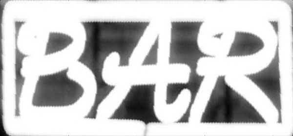
and we just need to slice the image to the new width and height (w and h):

dst = dst[:int(h)+1, :int(w)+1]
plt.imshow(dst)
plt.show()