Drawing conics in Matplotlib

Plotting conic sections in Matplotlib may seem easy, but it can get complicated if we use matplotlib.pyplot.plot. Especially if we attempt o draw a conic not in its standard position (except for the hyperbola). There are some tricks we can use, like plotting in two parts for circles, ellipses and parabolas, and masking values where the function is not defined for hyperbolas.

Instead we can create a two-dimensional Cartesian plane and draw the contour corresponding to the conic algebraic function.

Let's star importing the modules and setting some aesthetic properties:

import numpy as np
import matplotlib as mpl
import matplotlib.pyplot as plt

mpl.rcParams['lines.color'] = 'k'
mpl.rcParams['axes.prop_cycle'] = mpl.cycler('color', ['k'])

For the following examples we'll use the same plane as follows:

x = np.linspace(-9, 9, 400)
y = np.linspace(-5, 5, 400)
x, y = np.meshgrid(x, y)

Take into account that numpy.meshgrid creates a grid replicating the first array horizontally and the second array vertically, in the same way of MATLAB's meshgrid. Do not confuse with numpy.mgrid, which result will be a transposed meshgrid.

To simplify our examples, let's define a function to plot the origin axes:

def axes():
    plt.axhline(0, alpha=.1)
    plt.axvline(0, alpha=.1)

Parabolas

Parabolas in standard position follow an equation of the form

\[ y^2 = 4ax, \quad \text{with}\ a>0. \]

Using matplotlib.pyplot.contour and arranging \(4ax\) to the left hand side we can draw a parabola in standard position as:

a = .3
axes()
plt.contour(x, y, (y**2 - 4*a*x), [0], colors='k')
plt.show()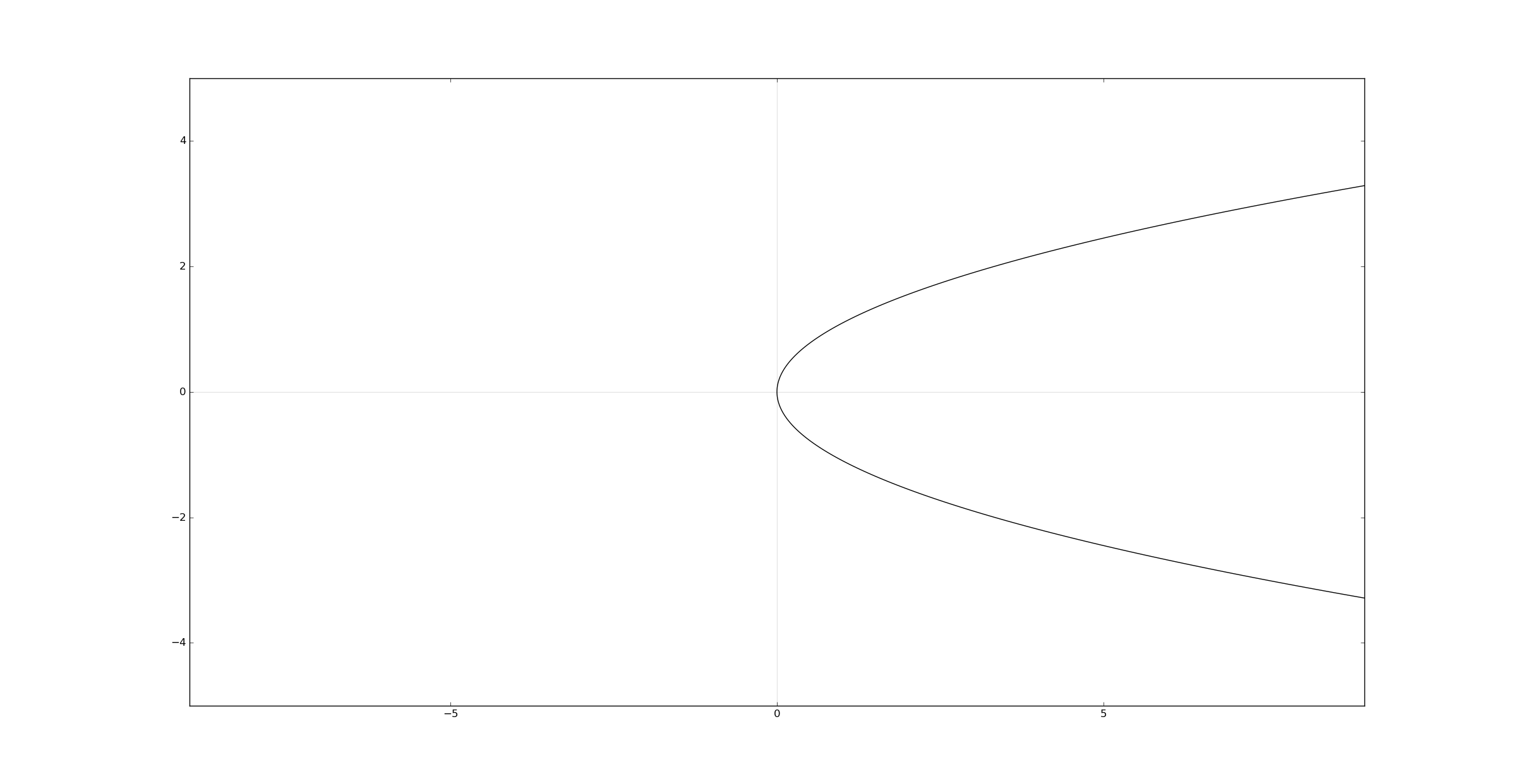

The focus is \((a,0)\) and the directrix is \(x=-a\),

axes()
plt.contour(x, y, (y**2 - 4*a*x), [0], colors='k', alpha=.1)
# Focus.
plt.plot(a, 0, '.')
# Directrix.
plt.axvline(-a)
plt.show()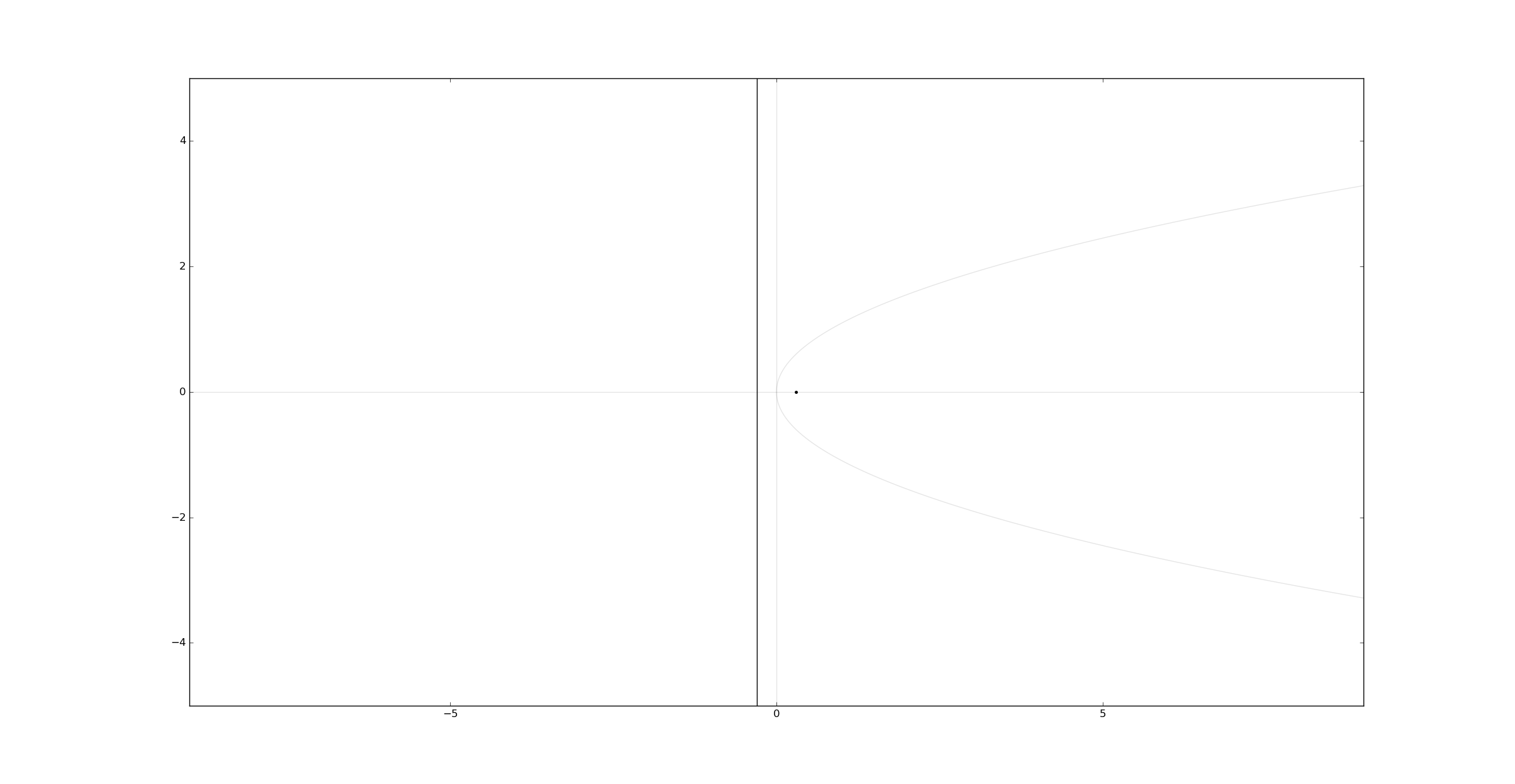

To define a parabola in a non-standard position is has to follow the form

\[ Ax^2 + Bxy + Cy^2 + Dx + Ey + F = 0, \quad \text{where}\ B^2 - 4AC = 0. \]

A parabola in a non-standard position:

a, b, c, d, e, f = 1, -2, 1, 2, 2, -10
assert b**2 - 4*a*c == 0
axes()
plt.contour(x, y,(a*x**2 + b*x*y + c*y**2 + d*x + e*y + f), [0], colors='k')
plt.show()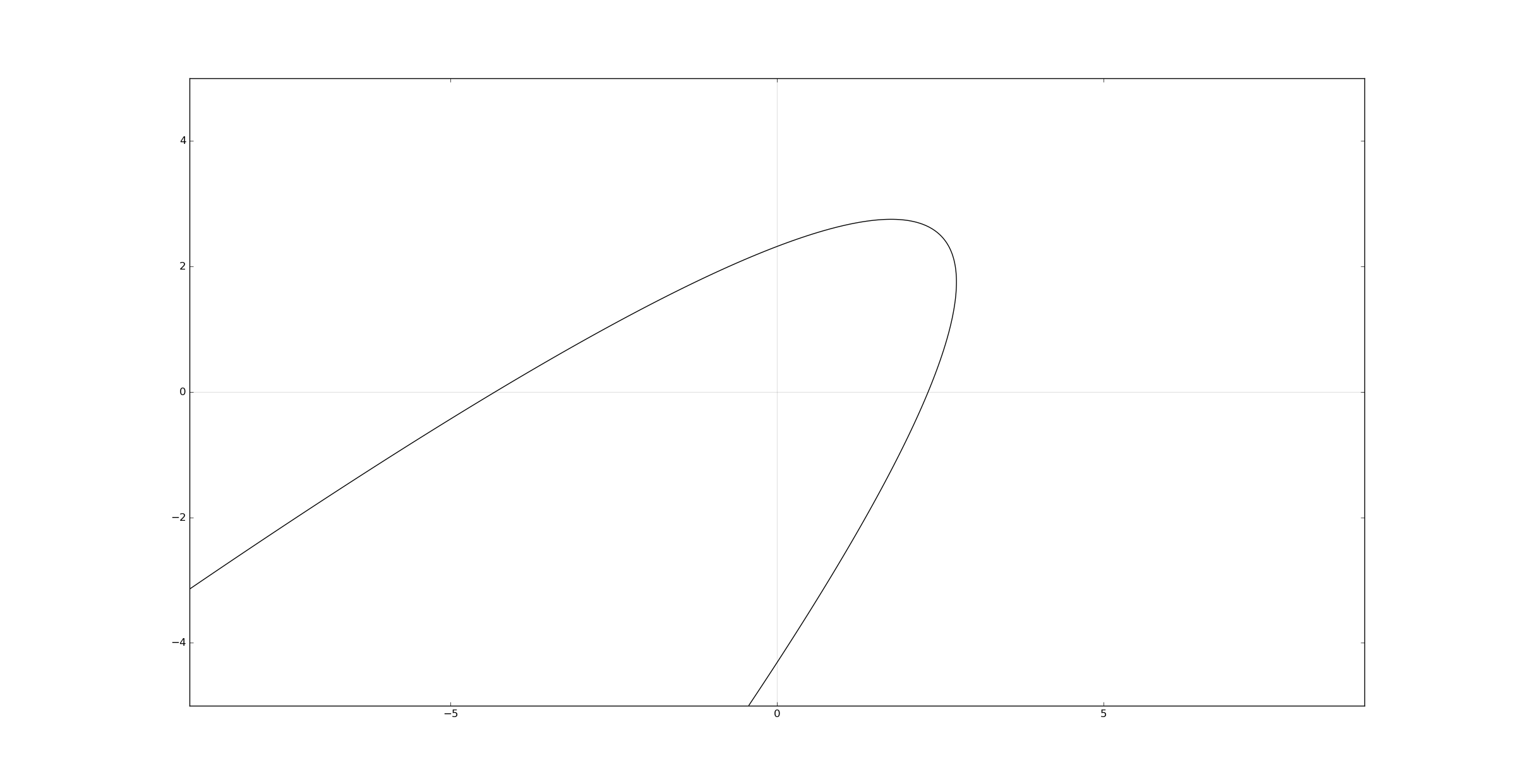

Ellipses and circles

Ellipses in standard position follow an equation of the form

\[ {x^2 \over a^2} + {y^2 \over b^2} = 1, \quad \text{where}\ a > b > 0. \]

In the case of the circles, \(a=b\).

A circle in standard position:

a = 2.
b = 2.
axes()
plt.contour(x, y,(x**2/a**2 + y**2/b**2), [1], colors='k')
plt.show()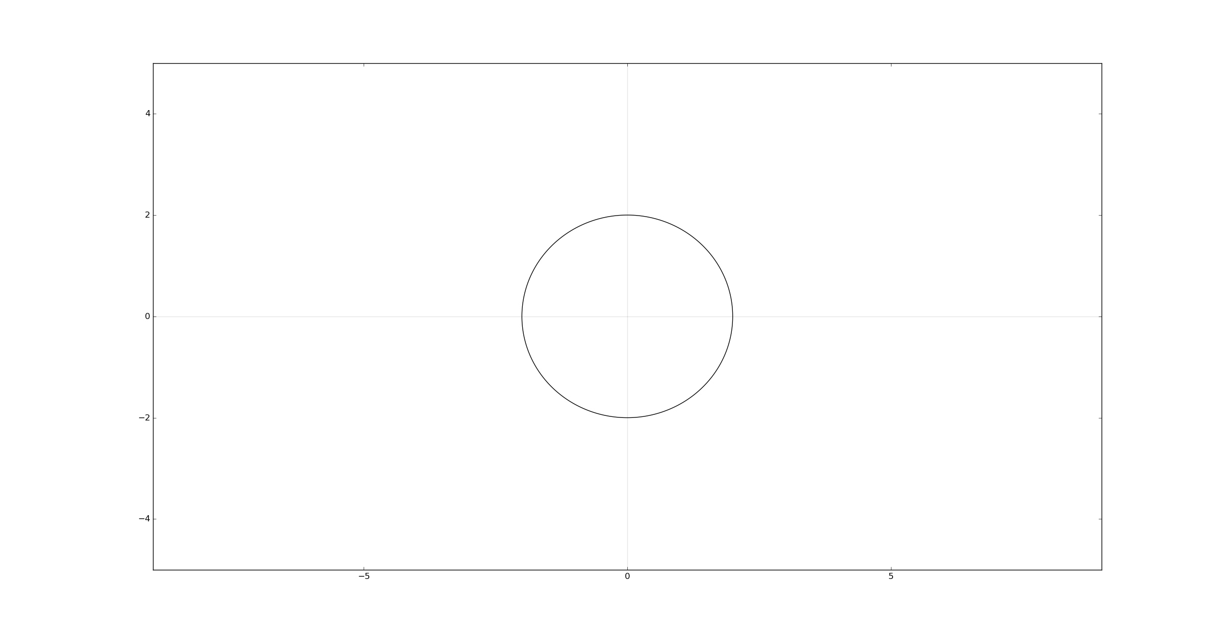

A ellipse in standard position:

a = 4.
b = 2.
axes()
plt.contour(x, y,(x**2/a**2 + y**2/b**2), [1], colors='k')
plt.show()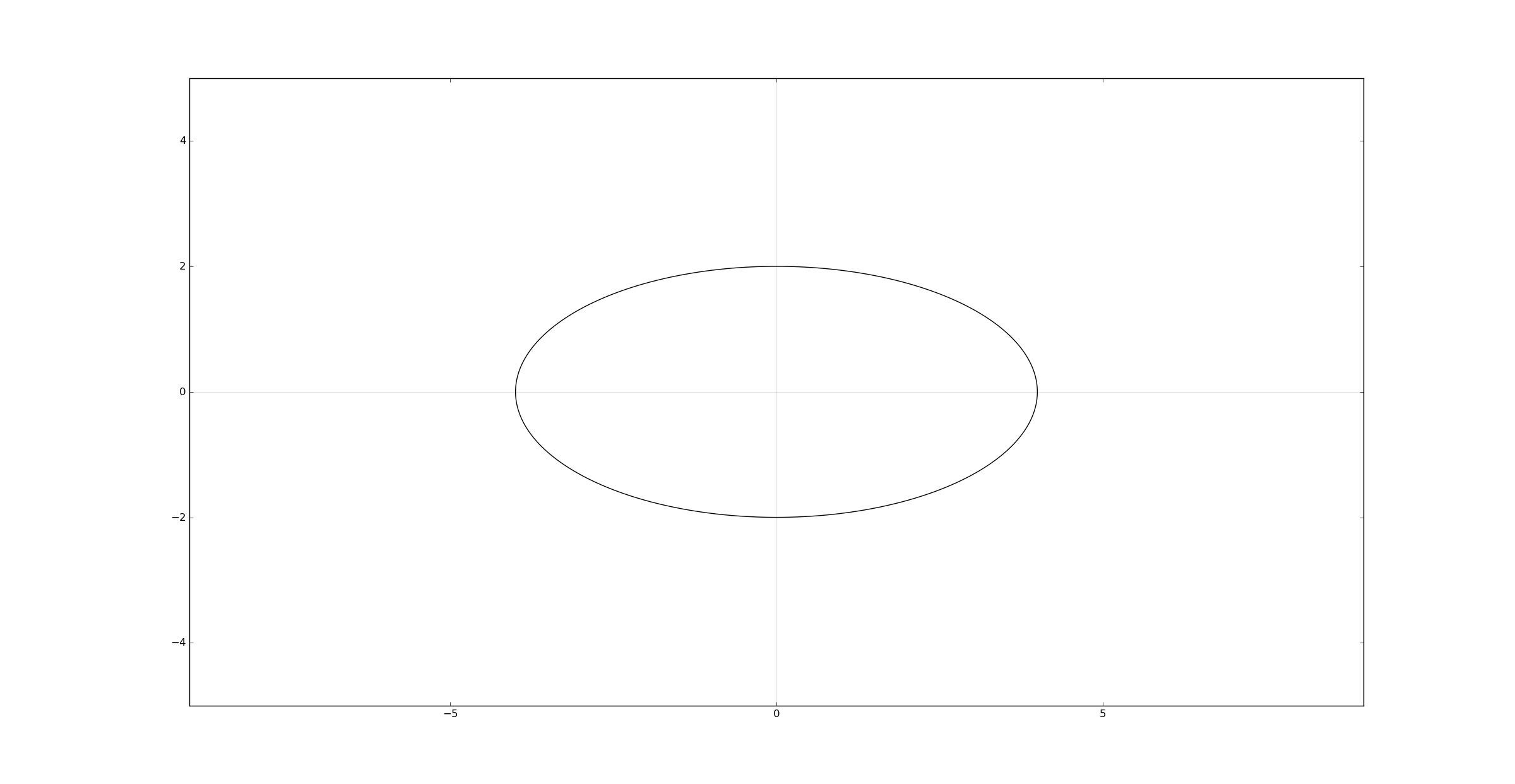

In the case of the parabola the eccentricity \(e=1\). For ellipses, the eccentricity \(0 < e < 1\) and it is defined as

\[ e = \sqrt{1 - {b^2 \over a^2}}. \]

The foci are \((\pm ae,0)\) and the directrices are \(x=\pm {a \over e}\),

axes()
plt.contour(x, y,(x**2/a**2 + y**2/b**2), [1], colors='k', alpha=.1)
# Eccentricity.
e = np.sqrt(1 - b**2/a**2)
# Foci.
plt.plot(a*e, 0, '.', -a*e, 0, '.')
# Directrices.
plt.axvline(a/e)
plt.axvline(-a/e)
plt.show()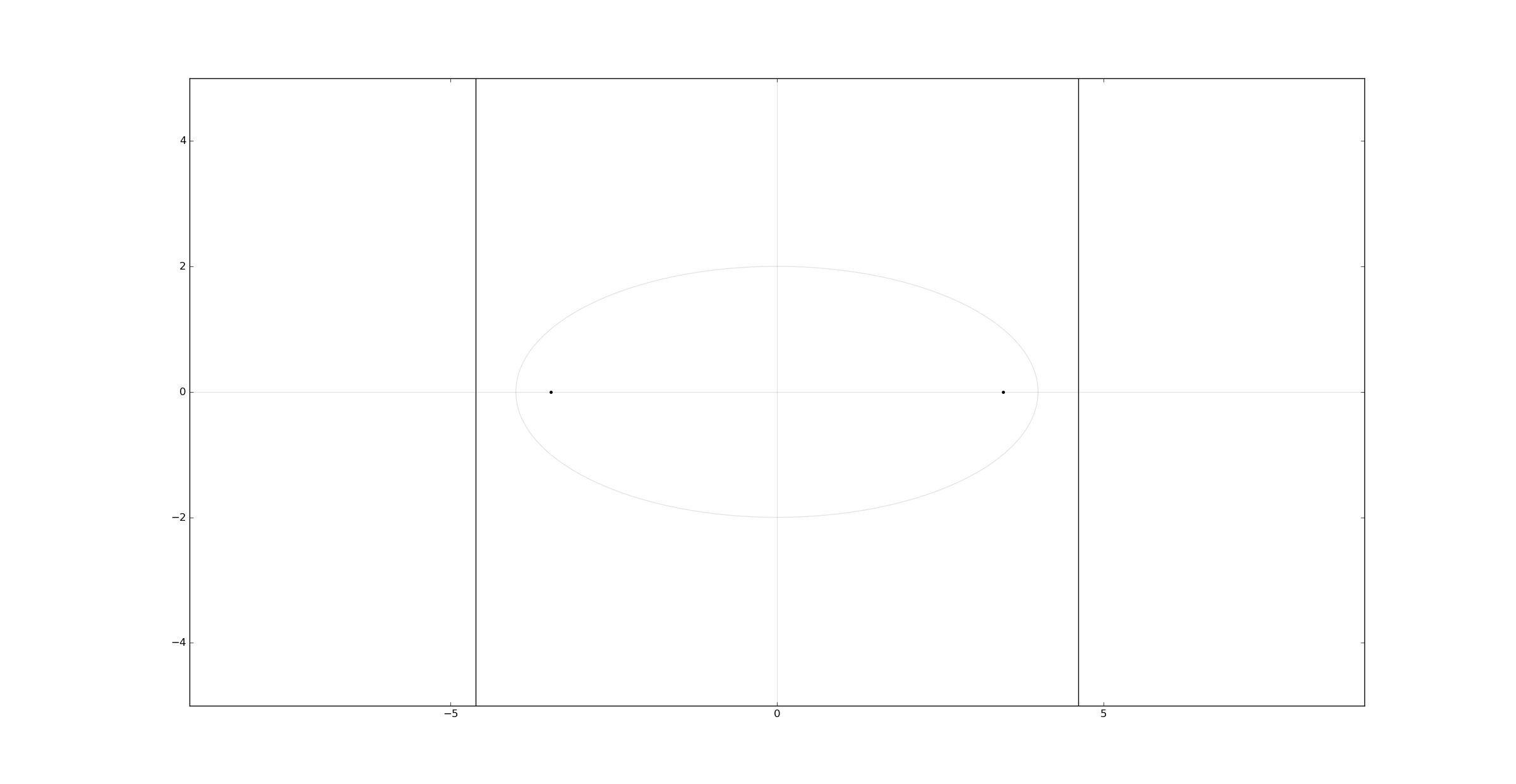

An ellipsis in a non-standard position has an equation in the same form of the parabola, but with the requisite

\[ B^2 - 4AC < 0, \]

a, b, c, d, e, f = 4, -5, 2, 4, -3, -3
assert b**2 - 4*a*c < 0
axes()
plt.contour(x, y,(a*x**2 + b*x*y + c*y**2 + d*x + e*y + f), [0], colors='k')
plt.show()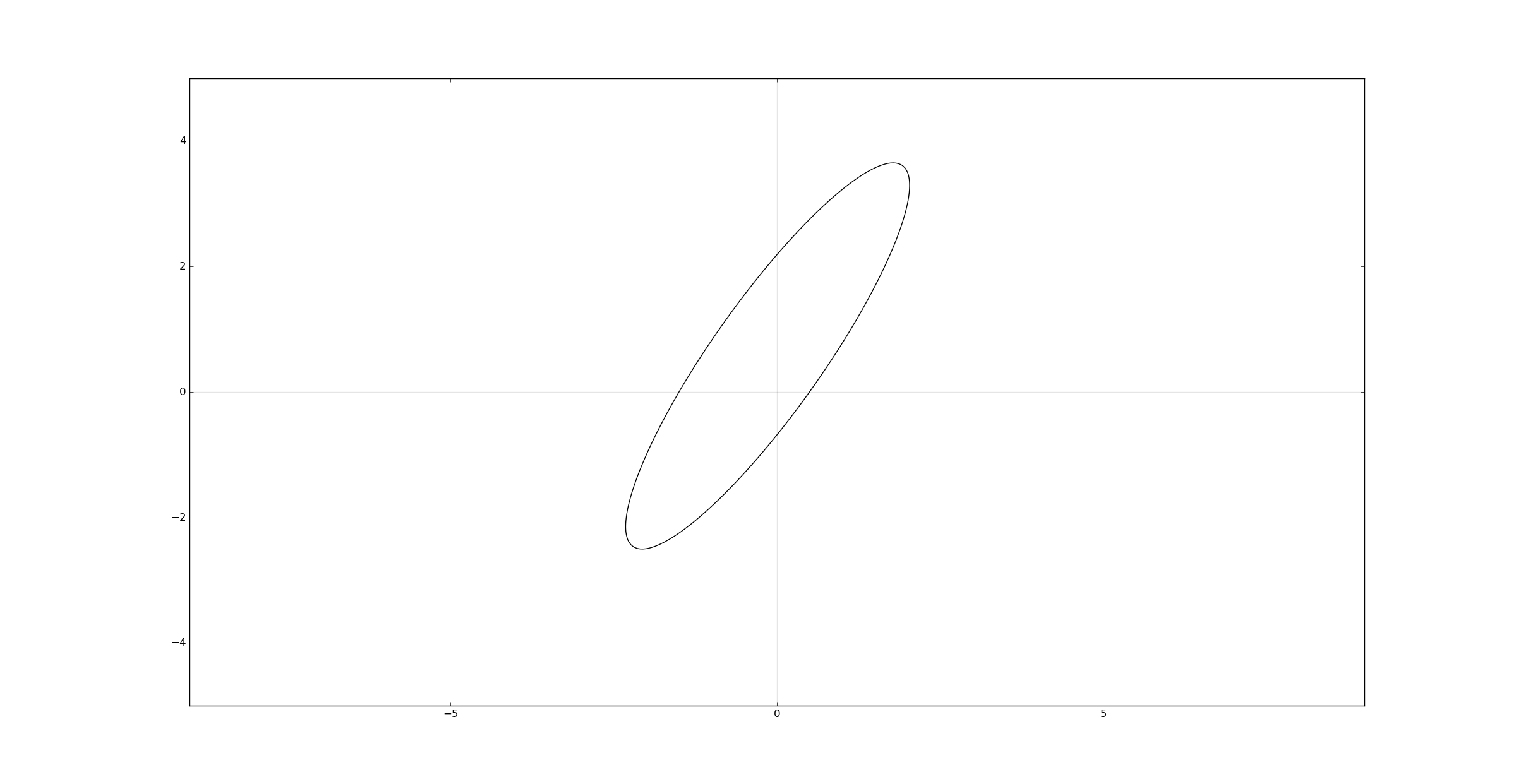

Hyperbolas

Hyperbolas in standard position follow an equation of the form

\[ {x^2 \over a^2} - {y^2 \over b^2} = 1, \quad \text{where}\ a, b > 0. \]

An hyperbola in standard position:

a = 2.
b = 1.
axes()
plt.contour(x, y,(x**2/a**2 - y**2/b**2), [1], colors='k')
plt.show()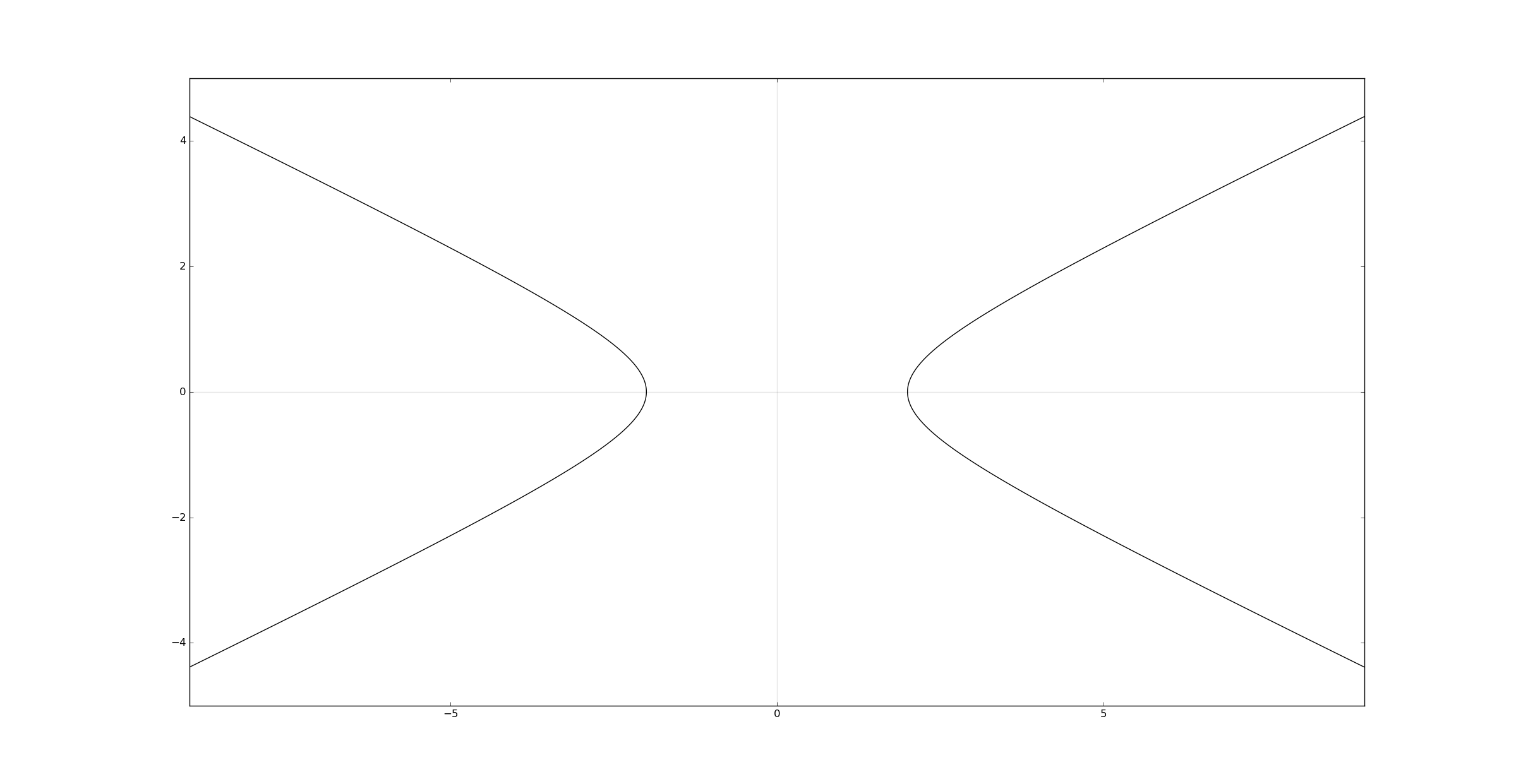

The eccentricity \(e > 1\) is defined as

\[ e = \sqrt{1 + {b^2 \over a^2}}, \]

The foci and directrices are the same as the ellipsis and the asymptotes can be found at \(y = \pm {b \over a}x\),

axes()
plt.contour(x, y,(x**2/a**2 - y**2/b**2), [1], colors='k', alpha=.1)
# Eccentricity.
e = np.sqrt(1 + b**2/a**2)
# Foci.
plt.plot(a*e, 0, '.', -a*e, 0, '.')
# Directrices.
plt.axvline(a/e)
plt.axvline(-a/e)
# Asymptotes.
plt.plot(x[0,:], b/a*x[0,:], '--')
plt.plot(x[0,:], -b/a*x[0,:], '--')
plt.show()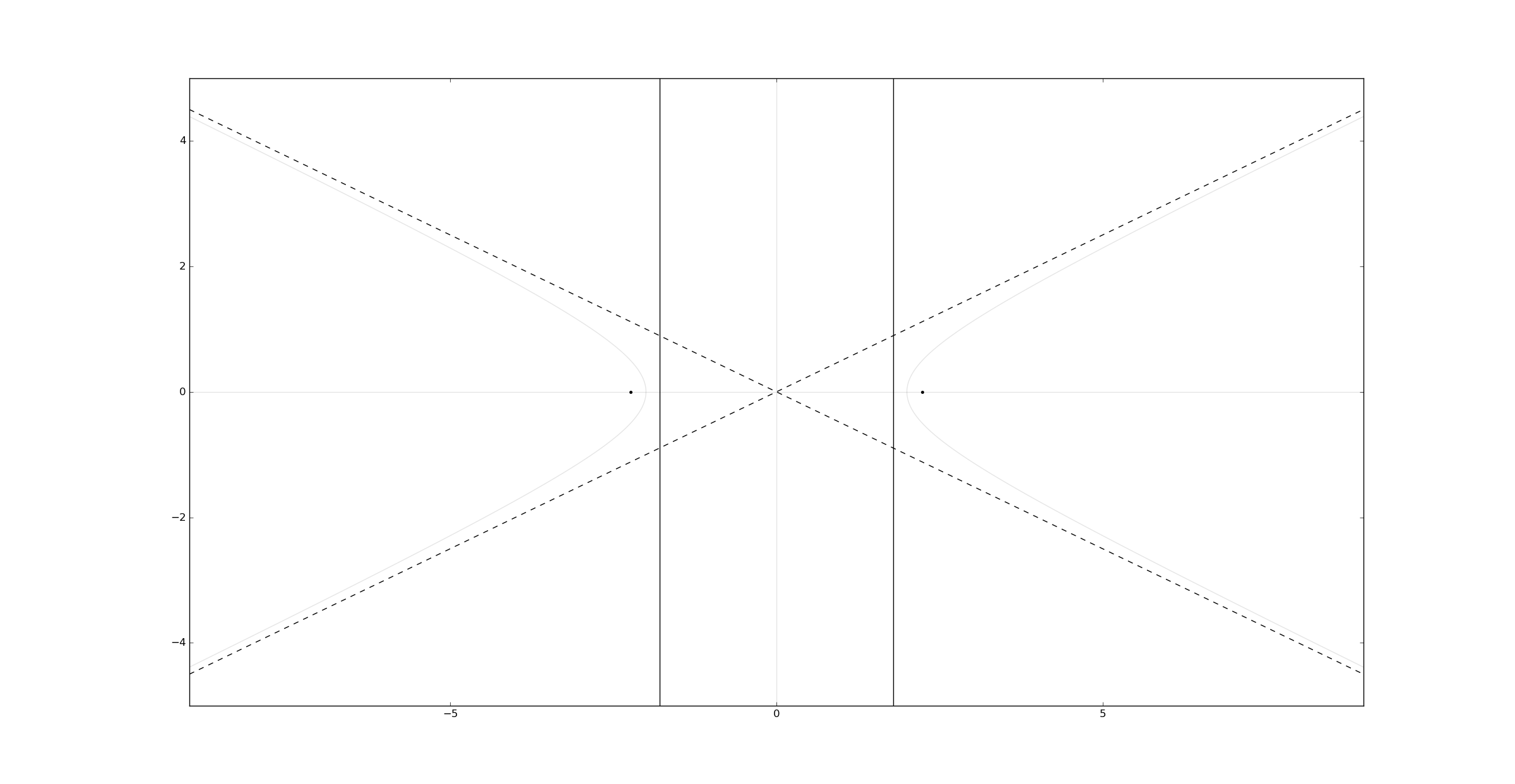

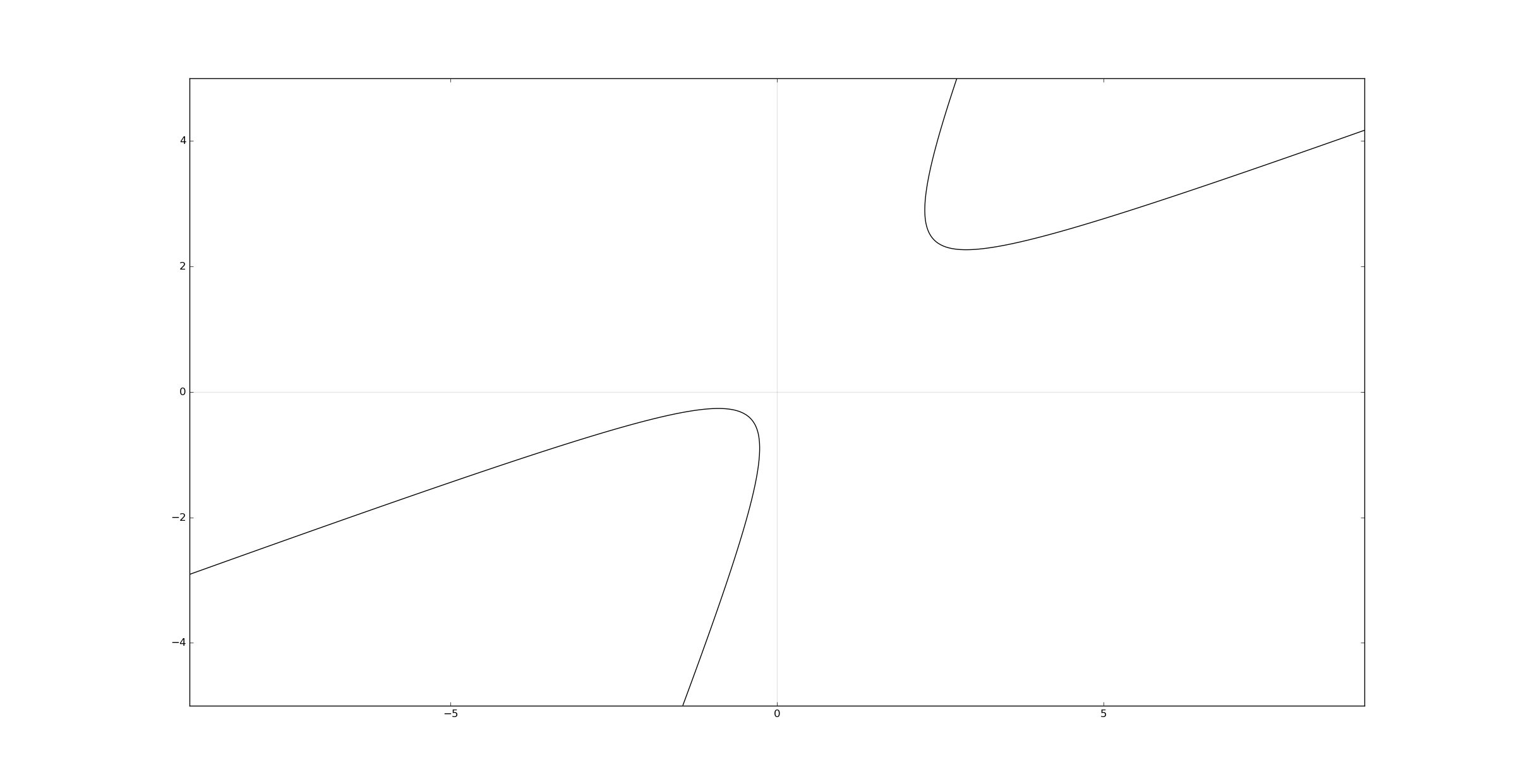
An hyperbola in a non-standard position has an equation in the same form as before with the requisite

\[ B^2 - 4AC > 0, \]

a, b, c, d, e, f = 1, -3, 1, 1, 1, 1
assert b**2 - 4*a*c > 0
axes()
plt.contour(x, y,(a*x**2 + b*x*y + c*y**2 + d*x + e*y + f), [0], colors='k')
plt.show()